Calibration Curves and Area Under the Curve

Understanding the mathematical intuition behind calibration curves and related metrics helps clarify their diagnostic value in evaluating model reliability. This section outlines foundational concepts using simplified examples, progressing toward their real-world interpretation in model evaluation.

Calibration Curves and Area Interpretation

Calibration curves visualize how well predicted probabilities align with actual outcomes. A perfectly calibrated model lies along the diagonal line, where predicted probability equals observed frequency.

Below are two manual examples using toy functions to illustrate the concept of area under the calibration curve, a key component of metrics like Calibration AUC.

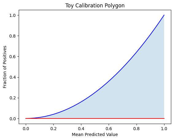
Example 1: Calibration with y = x²

This function simulates underconfident predictions, where the model consistently underestimates risk.

To compute the calibration area under this curve from ( x = 0 ) to ( x = 1 ):

\[\text{Area} = \int_0^1 x^2 \, dx\]

Solution:

\[\left[ \frac{x^3}{3} \right]_0^1 = \frac{1}{3}\]

The area under the ideal calibration line (diagonal) is:

\[\int_0^1 x \, dx = \left[ \frac{x^2}{2} \right]_0^1 = \frac{1}{2}\]

So, the polygonal calibration AUC becomes:

\[\frac{1}{2} - \frac{1}{3} = \frac{1}{6}\]

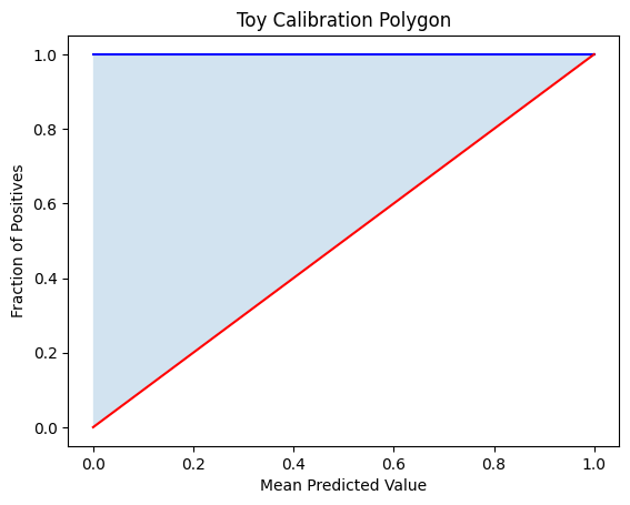
Example 2: Calibration with y = x² + 4x

This toy example models overconfident predictions, where the model consistently overshoots risk.

To calculate the area under the curve from ( x = 0 ) to ( x = 1 ), we compute the definite integral:

\[\text{Area} = \int_0^1 (x^2 + 4x) \, dx\]

Solution:

We split the integral into two separate parts:

\[\int_0^1 (x^2 + 4x) \, dx = \int_0^1 x^2 \, dx + \int_0^1 4x \, dx\]

First Integral:

\[\int_0^1 x^2 \, dx = \left[ \frac{x^3}{3} \right]_0^1 = \frac{1^3}{3} - \frac{0^3}{3} = \frac{1}{3}\]

Second Integral:

\[\int_0^1 4x \, dx = 4 \int_0^1 x \, dx = 4 \left[ \frac{x^2}{2} \right]_0^1 = 4 \left( \frac{1^2}{2} - \frac{0^2}{2} \right) = 4 \cdot \frac{1}{2} = 2\]

Final Answer:

\[\int_0^1 (x^2 + 4x) \, dx = \frac{1}{3} + 2 = \frac{7}{3}\]

This result represents the total area under the curve \(y = x^2 + 4x\) over the interval \([0, 1]\). If comparing against the ideal calibration line \(( y = x)\), you would subtract the diagonal area \(( \frac{1}{2})\) to isolate the calibration polygon AUC.

Note

In real calibration plots, the area is bounded within [0,1] on both axes. This example is meant to illustrate the mechanics of integration over a custom curve.