iPython Notebooks

Binary Classification Examples

Google Colab Notebooks

Binary Classification + KFold Example: Titanic Dataset - Categorical Data

Binary Classification: AIDS Clinical Trials - Numerical Data

Binary Classification: Imbalanced Learning

HTML Files

Binary Classification + KFold Example: Titanic Dataset - Categorical Data

Binary Classification: AIDS Clinical Trials HTML File

Binary Classification: Imbalanced Learning

Regression Example

Google Colab Notebook

Redfin Real Estate - Los Angeles Data Colab Notebook

HTML File

Redfin Real Estate - Los Angeles Data HTML File

Note

This class is designed to be flexible and can be extended to include additional functionalities or custom metrics.
It is essential to properly configure the parameters during initialization to suit the specific requirements of your machine learning task.
Ensure that all dependencies are installed and properly imported before using the Model class from the model_tuner library.

Input Parameters

class Model(name, estimator_name, estimator, model_type, calibrate=False, kfold=False, imbalance_sampler=None, train_size=0.6, validation_size=0.2, test_size=0.2, stratify_y=False, stratify_cols=None, grid=None, scoring=['roc_auc'], n_splits=10, random_state=3, n_jobs=1, display=True, randomized_grid=False, n_iter=100, pipeline_steps=[], boost_early=False, feature_selection=False, class_labels=None, multi_label=False, calibration_method='sigmoid', custom_scorer=[], bayesian=False)

A class for building, tuning, and evaluating machine learning models, supporting both classification and regression tasks, as well as multi-label classification.

Parameters:

name (str) – A unique name for the model, helpful for tracking outputs and logs.
estimator_name (str) – Prefix for the estimator in the pipeline, used for setting parameters in tuning (e.g., estimator_name + __param_name).
estimator (object) – The machine learning model to be trained and tuned.
model_type (str) – Specifies the type of model, must be either classification or regression.
calibrate (bool, optional) – Whether to calibrate the model’s probability estimates. Default is False.
kfold (bool, optional) – Whether to perform k-fold cross-validation. Default is False.
imbalance_sampler (object, optional) – An imbalanced data sampler from the imblearn library, e.g., RandomUnderSampler or RandomOverSampler.
train_size (float, optional) – Proportion of the data to be used for training. Default is 0.6.
validation_size (float, optional) – Proportion of the data to be used for validation. Default is 0.2.
test_size (float, optional) – Proportion of the data to be used for testing. Default is 0.2.
stratify_y (bool, optional) – Whether to stratify by the target variable during data splitting. Default is False.
stratify_cols (str, list, or pandas.DataFrame, optional) – Columns to use for stratification during data splitting. Can be a single column name (as a string), a list of column names (as strings), or a DataFrame containing the columns for stratification. Default is None.
grid (list of dict) – Hyperparameter grid for model tuning, supporting both regular and Bayesian search.
scoring (list of str) – List of scoring metrics for evaluation, e.g., ["roc_auc", "accuracy"].
n_splits (int, optional) – Number of splits for k-fold cross-validation. Default is 10.
random_state (int, optional) – Seed for random number generation to ensure reproducibility. Default is 3.
n_jobs (int, optional) – Number of parallel jobs to run for model fitting. Default is 1.
display (bool, optional) – Whether to print messages during the tuning and training process. Default is True.
randomized_grid (bool, optional) – Whether to use randomized grid search. Default is False.
n_iter (int, optional) – Number of iterations for randomized grid search. Default is 100.
pipeline_steps (list, optional) – List of steps for the pipeline, e.g., preprocessing and feature selection steps. Default is [].
boost_early (bool, optional) – Whether to enable early stopping for boosting algorithms like XGBoost. Default is False.
feature_selection (bool, optional) – Whether to enable feature selection. Default is False.
class_labels (list, optional) – List of labels for multi-class classification. Default is None.
multi_label (bool, optional) – Whether the task is a multi-label classification problem. Default is False.
calibration_method (str, optional) – Method for calibration; options include sigmoid and isotonic. Default is sigmoid.
custom_scorer (dict, optional) – Dictionary of custom scoring functions, allowing additional metrics to be evaluated. Default is [].
bayesian (bool, optional) – Whether to perform Bayesian hyperparameter tuning using BayesSearchCV. Default is False.

Raises:

ImportError – If the bootstrapper module is not found or not installed.
ValueError – Raised for various issues, such as: - Invalid model_type value. The model_type must be explicitly specified as either classification or regression. - Invalid hyperparameter configurations or mismatched X and y shapes.
AttributeError – Raised if an expected pipeline step is missing, or if self.estimator is improperly initialized.
TypeError – Raised when an incorrect parameter type is provided, such as passing None instead of a valid object.
IndexError – Raised for indexing issues, particularly in confusion matrix formatting functions.
KeyError – Raised when accessing dictionary keys that are not available, such as missing scores in self.best_params_per_score.
RuntimeError – Raised for unexpected issues during model fitting or transformations that do not fit into the other exception categories.

Key Methods and Functionalities

`init(...)`

Initializes the model tuner with configurations, including estimator, cross-validation settings, scoring metrics, pipeline steps, feature selection, imbalance sampler, Bayesian search, and model calibration options.

`reset_estimator()`

reset_estimator()

Resets the estimator and pipeline configuration.

Description:

This function reinitializes the estimator attribute of the class based on the current pipeline configuration.
If pipeline_steps are defined, it creates a new pipeline using self.PipelineClass and a deep copy of the steps.
If pipeline_steps are not defined, it resets the estimator to a single-step pipeline containing the original estimator.

Behavior:

If self.pipeline_steps is not empty:
- Creates a pipeline using the defined steps.
If self.pipeline_steps is empty:
- Resets the estimator to a single-step pipeline with the original estimator.

Attributes Used:

self.pipeline_steps: The steps of the pipeline (if defined).
self.PipelineClass: The class used to construct pipelines.
self.estimator_name: The name of the primary estimator step.
self.original_estimator: The original estimator to be reset.

Output:

The function updates the self.estimator attribute and does not return a value.

Notes:

This function is intended for internal use as a helper function to manage pipeline and estimator states.
Ensures that the pipeline or estimator is always in a valid state after modifications or resets.

`process_imbalance_sampler()`

process_imbalance_sampler(X_train, y_train)

Processes the imbalance sampler, applying it to resample the training data.

Parameters:

X_train (pandas.DataFrame or array-like) – Training features to be resampled.
y_train (pandas.Series or array-like) – Training target labels to be resampled.

Raises:

KeyError – Raised if the resampler step is missing in the pipeline.
ValueError – Raised if X_train or y_train are incompatible with the pipeline or resampler.

Output:

Prints the class distribution of y_train after resampling.
Does not modify the original X_train or y_train.

Description:

This function applies an imbalance sampler to resample the training data, ensuring the target distribution is balanced.
If preprocessing steps are defined in the pipeline, they are applied to the training features before resampling.
Prints the distribution of y_train after resampling to provide visibility into the balance of classes.

Behavior:

If preprocessing steps exist (self.pipeline_steps):
- Applies preprocessing to X_train using the preprocessing pipeline obtained from get_preprocessing_pipeline().
Clones the resampler step from the pipeline to ensure independent operation.
Resamples the training data using the cloned resampler, modifying the distribution of y_train.

Attributes Used:

self.pipeline_steps: Indicates whether preprocessing steps are defined.
self.get_preprocessing_pipeline(): Retrieves the preprocessing pipeline (if available).
self.estimator.named_steps["resampler"]: The resampler to apply for balancing the target classes.

Note

The function assumes that the pipeline includes a valid resampler step under named_steps.
Ensures compatibility with pandas.DataFrame and array-like structures for y_train.
Prints the class distribution of y_train after resampling for user awareness.

`calibrateModel()`

calibrateModel(X, y, score=None)

Calibrates the model with cross-validation support and configurable calibration methods, improving probability estimates.

Parameters:

X (pandas.DataFrame or array-like) – Feature set used for model calibration.
y (pandas.Series or array-like) – Target set corresponding to X.
score (str or list of str, optional) – Optional scoring metric(s) for evaluating the calibration. Default is None.

Raises:

ValueError – Raised if incompatible parameters (e.g., invalid scoring metric) are passed.
KeyError – Raised if required attributes or parameters are missing.

Description:

Supports model calibration with both k-fold cross-validation and a pre-split train-validation-test workflow.
Uses CalibratedClassifierCV for calibration with methods such as sigmoid or isotonic (defined by self.calibration_method).
Handles cases where imbalance sampling or early stopping is applied during training.
Provides additional support for CPU/GPU device management if applicable.

Behavior:

With K-Fold Cross-Validation:
- Resets the estimator to avoid conflicts with pre-calibrated models.
- Calibrates the model using k-fold splits with the configured calibration method.
- Optionally evaluates calibration using the provided scoring metric(s).
- Generates and prints confusion matrices for each fold (if applicable).
Without K-Fold Cross-Validation:
- Performs a train-validation-test split using train_val_test_split.
- Resets the estimator and applies preprocessing or imbalance sampling if configured.
- Fits the model on training data, with or without early stopping.
- Calibrates the pre-trained model on the test set and evaluates calibration results.

Attributes Used:

self.kfold: Indicates whether k-fold cross-validation is enabled.
self.calibrate: Determines whether calibration is applied.
self.calibration_method: Specifies the calibration method (e.g., sigmoid or isotonic).
self.best_params_per_score: Stores the best parameters for each scoring metric.
self.n_splits: Number of splits for cross-validation.
self.stratify_y, self.stratify_cols: Used for stratified train-validation-test splitting.
self.imbalance_sampler: Indicates if an imbalance sampler is applied.
self.boost_early: Enables early stopping during training.

Output:

Modifies the class attribute self.estimator to include the calibrated model.
Generates calibration reports and scoring metrics if applicable.
Prints performance metrics (e.g., scores and confusion matrices) for the calibrated model.

Note

When score is provided, the function evaluates calibration using the specified metric(s).
Requires the estimator to be compatible with CalibratedClassifierCV.
Handles both balanced and imbalanced datasets with preprocessing support.

Get train, val, test data

Description:

These functions return subsets of the dataset (features and labels) based on predefined indices stored in the class attributes:
- self.X_train_index and self.y_train_index for training data.
- self.X_valid_index and self.y_valid_index for validation data.
- self.X_test_index and self.y_test_index for test data.
Designed to work with pandas.DataFrame and pandas.Series objects.

`get_train_data()`

get_train_data(X, y)

Retrieves the training data based on specified indices.

Parameters:

X (pandas.DataFrame) – Full dataset containing features.
y (pandas.Series) – Full dataset containing target labels.

Returns:

A tuple containing the training features and labels.

Return type:

tuple of (pandas.DataFrame, pandas.Series)

`get_valid_data()`

get_valid_data(X, y)

Retrieves the validation data based on specified indices.

Parameters:

X (pandas.DataFrame) – Full dataset containing features.
y (pandas.Series) – Full dataset containing target labels.

Returns:

A tuple containing the validation features and labels.

Return type:

tuple of (pandas.DataFrame, pandas.Series)

`get_test_data()`

get_test_data(X, y)

Retrieves the test data based on specified indices.

Parameters:

X (pandas.DataFrame) – Full dataset containing features.
y (pandas.Series) – Full dataset containing target labels.

Returns:

A tuple containing the test features and labels.

Return type:

tuple of (pandas.DataFrame, pandas.Series)

Note

These methods assume that the indices (e.g., self.X_train_index) are defined and valid.
The methods return subsets of the provided X and y data by indexing the rows based on the stored indices.
Useful for workflows where train, validation, and test splits are dynamically managed or predefined.

`calibrate_report()`

calibrate_report(X, y, score=None)

Generates a calibration report, including a confusion matrix and classification report.

Parameters:

X (pandas.DataFrame or array-like) – Features dataset for validation.
y (pandas.Series or array-like) – True labels for the validation dataset.
score (str, optional) – Optional scoring metric name to include in the report. Default is None.

Raises:

ValueError – Raised if the provided X or y are incompatible with the model or metrics.

Description:

This method evaluates the performance of a calibrated model on the validation dataset.
Generates and prints: - A confusion matrix, with support for multi-label classification if applicable. - A classification report summarizing precision, recall, and F1-score for each class.

Behavior:

Calls the predict method to obtain predictions for the validation dataset.
Uses confusion_matrix or multilabel_confusion_matrix based on the value of self.multi_label to compute the confusion matrix.
Prints a labeled confusion matrix using the _confusion_matrix_print() function.
Generates a classification report using classification_report from sklearn.metrics and assigns it to the self.classification_report attribute.

Output:

Prints the following to the console:
- The confusion matrix with labels.
- The classification report.
- A separator line for readability.
Updates the attribute self.classification_report with the generated classification report.

Note

If the model is multi-label, a confusion matrix is generated for each label.
The optional score parameter can be used to specify and display a scoring metric in the report heading.
Designed to work with models that support binary, multi-class, or multi-label predictions.

`fit()`

fit(X, y, validation_data=None, score=None)

Fits the model to training data and, if applicable, tunes thresholds and performs early stopping. Allows feature selection and processing steps as part of the pipeline.

Parameters:

X (pandas.DataFrame or array-like) – Training features.
y (pandas.Series or array-like) – Training target labels.
validation_data (tuple of (pandas.DataFrame, pandas.Series), optional) – Tuple containing validation features and labels. Required for early stopping. Default is None.
score (str, optional) – Optional scoring metric to guide the fitting process. Default is None.

Raises:

ValueError – Raised if invalid scoring metrics or parameters are provided.

Description:

This method trains the model with support for both k-fold cross-validation and single train-validation-test workflows.
If feature selection or preprocessing steps are configured, they are applied before fitting.
For certain estimators, early stopping is supported when validation data is provided.
The method dynamically sets model parameters based on tuning results for the specified or default scoring metric.

Behavior:

With K-Fold Cross-Validation:

Resets the estimator and fits the model using k-fold splits.

If a scoring metric is provided, applies it to guide the cross-validation.

Stores cross-validation results in the self.xval_output attribute.

Without K-Fold Cross-Validation:

Resets the estimator and applies feature selection or preprocessing if configured.

Fits the model on training data. If early stopping is enabled, uses validation data to monitor performance and stop training early.

Attributes Used:

self.kfold: Indicates whether k-fold cross-validation is enabled.
self.best_params_per_score: Stores tuned parameters for different scoring metrics.
self.feature_selection, self.pipeline_steps: Flags for feature selection and preprocessing steps.
self.imbalance_sampler: Specifies whether imbalance sampling is applied.
self.boost_early: Enables early stopping during training.
self.estimator_name: Name of the estimator in the pipeline.

Output:

Updates the class attribute self.estimator with the fitted model.
For k-fold cross-validation, stores results in self.xval_output.

Note

Early stopping requires both validation features and labels.
Feature selection and preprocessing steps are dynamically applied based on the pipeline configuration.
When a custom scoring metric is specified, it must match one of the predefined or user-defined metrics.

`return_metrics()`

return_metrics(X, y, optimal_threshold=False, model_metrics=False, print_threshold=False, return_dict=False, print_per_fold=False)

A flexible function to evaluate model performance by generating classification or regression metrics. It provides options to print confusion matrices, classification reports, and regression metrics, and supports optimal threshold display and dictionary outputs.

Parameters:

X (pandas.DataFrame or array-like) – The feature matrix for evaluation.
y (pandas.Series or array-like) – The target vector for evaluation.
optimal_threshold (bool, optional) – Whether to use the optimal threshold for predictions (classification only). Default is False.
model_metrics (bool, optional) – Whether to calculate and print detailed model metrics using report_model_metrics(). Default is False.
print_threshold (bool, optional) – Whether to print the optimal threshold used for predictions (classification only). Default is False.
return_dict (bool, optional) – Whether to return the metrics as a dictionary instead of printing them. Default is False.
print_per_fold (bool, optional) – For cross-validation, whether to print metrics for each fold. Default is False.

Returns:

A dictionary containing metrics if return_dict=True; otherwise, the metrics are printed.

Return type:

dict or None

Description:

The return_metrics() function is designed to be highly adaptable, allowing users to:

Print Classification Metrics: Displays a confusion matrix and the accompanying classification report when evaluating a classification model.
Print Regression Metrics: Outputs standard regression metrics (e.g., R², Mean Absolute Error) when evaluating a regression model.
Report Detailed Model Metrics: By setting model_metrics=True, the function invokes report_model_metrics() to provide detailed insights into metrics like precision, recall, and AUC-ROC.
Display the Optimal Threshold: Setting print_threshold=True displays the threshold value used for classification predictions, particularly when an optimal threshold has been tuned.
Return Results as a Dictionary: If return_dict=True, the metrics are returned in a structured dictionary, allowing users to programmatically access the results. This is especially useful for further analysis or logging.

Behavior:

Classification Models:
- Generates and prints a confusion matrix.
- Prints a detailed classification report, including precision, recall, F1-score, and accuracy.
- Optionally prints additional model metrics and the optimal threshold.
Regression Models:
- Outputs standard regression metrics such as R², Mean Absolute Error, and Root Mean Squared Error.
Cross-Validation:
- For k-fold validation, the function aggregates metrics across folds and prints the averaged results. If print_per_fold=True, metrics for each fold are also printed in addition to the averaged results.

Output:

If return_dict=True, returns:
- Classification Models:
  - A dictionary with:
    - Classification Report: The classification report as a string.
    - Confusion Matrix: The confusion matrix as an array.
    - Best Features: (Optional) List of the top features if feature selection is enabled.
- Regression Models:
  - A dictionary with:
    - Regression Report: A dictionary of regression metrics.
    - Best Features: (Optional) List of the top features if feature selection is enabled.
If return_dict=False, prints the metrics directly to the console.

Examples:

## Example usage for validation metrics:
print("Validation Metrics")
model.return_metrics(
    X=X_valid,
    y=y_valid,
    optimal_threshold=True,
    print_threshold=True,
    model_metrics=True,
)
print()

## Example usage for test metrics:
print("Test Metrics")
model.return_metrics(
    X=X_test,
    y=y_test,
    optimal_threshold=True,
    print_threshold=True,
    model_metrics=True,
)
print()

Note

This function is suitable for both classification and regression models.
Supports cross-validation workflows by calculating metrics across multiple folds.
Enables users to programmatically access metrics via the dictionary output for custom analysis.

`predict()`

predict(X, y=None, optimal_threshold=False)

Makes predictions and predicts probabilities, allowing threshold tuning.

Parameters:

X (pandas.DataFrame or array-like) – The feature matrix for prediction.
y (pandas.Series or array-like, optional) – The true target labels, required only for k-fold predictions. Default is None.
optimal_threshold (bool, optional) – Whether to use an optimal classification threshold for predictions. Default is False.

Returns:

Predicted class labels or predictions adjusted by the optimal threshold.

Return type:

numpy.ndarray or array-like

Raises:

ValueError – Raised if invalid inputs or configurations are provided.

Description:

Predicts target values for the input data.
Supports both regression and classification tasks, with specific behavior for each:
- For regression: Direct predictions are returned, ignoring thresholds.
- For classification: Predictions are adjusted using an optimal threshold when enabled.
If k-fold cross-validation is active, performs predictions for each fold using cross_val_predict.

Behavior:

With K-Fold Cross-Validation:
- Returns predictions based on cross-validated folds.
Without K-Fold Cross-Validation:
- Uses the trained model’s predict() method.
- Applies the optimal threshold to adjust classification predictions, if specified.

Related Methods:

predict_proba(X, y=None):
- Predicts probabilities for classification tasks.
- Supports k-fold cross-validation using cross_val_predict with the method="predict_proba" option.

Note

Optimal thresholding is useful for fine-tuning classification performance metrics such as F1-score or precision-recall balance.
For classification, the threshold can be tuned for specific scoring metrics (e.g., ROC-AUC).
Works seamlessly with pipelines or directly with the underlying model.

`grid_search_param_tuning()`

grid_search_param_tuning(X, y, f1_beta_tune=False, betas=[1, 2])

Performs grid or Bayesian search parameter tuning, optionally tuning F-beta score thresholds for classification.

Parameters:

X (pandas.DataFrame or array-like) – The feature matrix for training and validation.
y (pandas.Series or array-like) – The target vector corresponding to X.
f1_beta_tune (bool, optional) – Whether to tune F-beta score thresholds during parameter search. Default is False.
betas (list of int, optional) – List of beta values to use for F-beta score tuning. Default is [1, 2].

Raises:

ValueError – Raised if the provided data or configurations are incompatible with parameter tuning.
KeyError – Raised if required scoring metrics are missing.

Description:

This method tunes hyperparameters for a model using grid search or Bayesian optimization.
Supports tuning F-beta thresholds for classification tasks.
Can handle both k-fold cross-validation and single train-validation-test workflows.

Behavior:

With K-Fold Cross-Validation:
- Splits data into k folds using kfold_split and performs parameter tuning.
- Optionally tunes thresholds for F-beta scores on validation splits.
Without K-Fold Cross-Validation:
- Performs a train-validation-test split using train_val_test_split.
- Applies preprocessing, feature selection, and imbalance sampling if configured.
- Tunes parameters and thresholds based on validation scores.

Attributes Used:

self.kfold: Indicates whether k-fold cross-validation is enabled.
self.scoring: List of scoring metrics used for evaluation.
self.best_params_per_score: Stores the best parameter set for each scoring metric.
self.grid: Parameter grid for tuning.
self.calibrate: Specifies whether the model calibration is enabled.
self.imbalance_sampler: Indicates if imbalance sampling is applied.
self.feature_selection: Specifies whether feature selection is applied.
self.pipeline_steps: Configuration for preprocessing steps.
self.boost_early: Enables early stopping during model training.
self.threshold: Stores tuned thresholds for F-beta score optimization.

Output:

Updates the class attribute self.best_params_per_score with the best parameters and scores for each metric.
Optionally updates self.threshold with tuned F-beta thresholds.
Prints best parameters and scores if self.display is enabled.

Note

Threshold tuning requires classification tasks and is not applicable for regression.
Early stopping is supported if self.boost_early is enabled and validation data is provided.
Works seamlessly with pipelines for preprocessing and feature selection.

`print_selected_best_features()`

print_selected_best_features(X)

Prints and returns the selected top K best features based on the feature selection step.

Parameters:: X (pandas.DataFrame or array-like) – The feature matrix used during the feature selection process.
Returns:: A list of the selected features or column indices.
Return type:: list
Raises:: AttributeError – Raised if the feature selection pipeline is not properly configured or trained.

Description:

This method retrieves the top K features selected by the feature selection pipeline.
Prints the names or column indices of the selected features to the console.
Returns the selected features as a list.

Behavior:

For DataFrames:
- Prints the names of the selected feature columns.
- Returns a list of column names corresponding to the selected features.
For Array-like Data:
- Prints the indices of the selected feature columns.
- Returns a list of column indices.

Attributes Used:

self.get_feature_selection_pipeline(): Retrieves the feature selection pipeline used for selecting features.

Output:

Prints the selected features or indices to the console.
Returns the selected features as a list.

Note

Assumes that a feature selection pipeline has been configured and trained prior to calling this method.
Designed to work with both pandas.DataFrame and array-like structures for feature matrices.

`tune_threshold_Fbeta()`

tune_threshold_Fbeta(score, y_valid, betas, y_valid_proba, kfold=False)

Tunes classification threshold for optimal F-beta score, balancing precision and recall across various thresholds.

Parameters:

score (str) – A label or name for the score used to store the best threshold.
y_valid (array-like of shape (n_samples,)) – Ground truth (actual) labels for the validation dataset.
betas (list of float) – A list of beta values to consider when calculating the F-beta score. Beta controls the balance between precision and recall.
y_valid_proba (array-like of shape (n_samples,)) – Predicted probabilities for the positive class in the validation dataset. Used to evaluate thresholds.
kfold (bool, optional) – If True, returns the best threshold for the given score. If False, updates the threshold attribute in place. Default is False.

Returns:

The best threshold for the given score if kfold is True, otherwise returns None.

Return type:

float or None

Raises:

ValueError – Raised if input arrays have mismatched dimensions or invalid beta values.
TypeError – Raised if invalid data types are passed for parameters.

Description:

This method identifies the optimal classification threshold for maximizing the F-beta score.
The F-beta score balances precision and recall, with beta determining the relative weight of recall.
Evaluates thresholds ranging from 0 to 1 (with a step size of 0.01) to find the best threshold for each beta value.

Behavior:

Threshold Evaluation:
- For each threshold, computes binary predictions and evaluates the resulting F-beta score.
- Penalizes thresholds leading to undesirable outcomes, such as excessive false positives compared to true negatives.
K-Fold Mode:
- If kfold=True, returns the optimal threshold without modifying class attributes.
Non K-Fold Mode:
- Updates the self.threshold attribute with the optimal threshold for the specified score.

Attributes Used:

self.threshold: Stores the optimal threshold for each scoring metric.
self.beta: Stores the beta value corresponding to the maximum F-beta score.

Notes:

The method iterates over thresholds and calculates F-beta scores for each beta value, identifying the best-performing threshold.
Penalizes thresholds where false positives exceed true negatives to ensure practical performance.
Designed to support models evaluated on binary classification tasks.

Example:

optimal_threshold = tune_threshold_Fbeta(
      score="roc_auc",
      y_valid=y_valid,
      betas=[0.5, 1, 2],
      y_valid_proba=model.predict_proba(X_valid)[:, 1],
      kfold=False,
)

`train_val_test_split()`

train_val_test_split(X, y, stratify_y=None, train_size=0.6, validation_size=0.2, test_size=0.2, random_state=3, stratify_cols=None)

Splits data into train, validation, and test sets, supporting stratification by specific columns or the target variable.

Parameters:

X (pandas.DataFrame or array-like) – The feature matrix to split.
y (pandas.Series or array-like) – The target vector corresponding to X.
stratify_y (pandas.Series or None, optional) – Specifies whether to stratify based on the target variable. Default is None.
train_size (float, optional) – Proportion of the data to allocate to the training set. Default is 0.6.
validation_size (float, optional) – Proportion of the data to allocate to the validation set. Default is 0.2.
test_size (float, optional) – Proportion of the data to allocate to the test set. Default is 0.2.
random_state (int, optional) – Random seed for reproducibility. Default is 3.
stratify_cols (list, pandas.DataFrame, or None, optional) – Columns to use for stratification, in addition to or instead of y. Default is None.

Returns:

A tuple containing train, validation, and test sets: (X_train, X_valid, X_test, y_train, y_valid, y_test).

Return type:

tuple of (pandas.DataFrame, pandas.Series)

Raises:

ValueError – Raised if the sizes for train, validation, and test do not sum to 1.0 or if invalid stratification keys are provided.

Description:

This function splits data into three sets: train, validation, and test.
Supports stratification based on the target variable (y) or specific columns (stratify_cols).
Ensures the proportions of the split sets are consistent with the specified train_size, validation_size, and test_size.

Behavior:

Combines stratify_cols and y (if both are provided) to create a stratification key.
Handles missing values in stratify_cols by filling with empty strings.
Uses a two-step splitting approach:
1. Splits data into train and combined validation-test sets.
2. Further splits the combined set into validation and test sets.

Attributes Used:

Handles configurations for stratification and proportional splitting.

Note

The sum of train_size, validation_size, and test_size must equal 1.0.
Stratification ensures the distribution of classes or categories is preserved across splits.
The function works seamlessly with both pandas.DataFrame and array-like data structures.

Example:

X_train, X_valid, X_test, y_train, y_valid, y_test = train_val_test_split(
    X=features,
    y=target,
    stratify_y=target,
    train_size=0.6,
    validation_size=0.20,
    test_size=0.20,
    random_state=42,
    stratify_cols=['category_column']
)

`get_best_score_params()`

get_best_score_params(X, y)

Retrieves the best hyperparameters for the model based on cross-validation scores for specified metrics.

Parameters:

X (pandas.DataFrame or array-like) – The feature matrix for training during hyperparameter tuning.
y (pandas.Series or array-like) – The target vector corresponding to X.

Returns:

None. Updates the class attributes with the best parameters and scores.

Return type:

None

Raises:

ValueError – Raised if self.grid or self.kf is not properly configured.
KeyError – Raised if scoring metrics are missing or invalid.

Description:

This method performs hyperparameter tuning using either grid search, randomized grid search, or Bayesian search.
Identifies the best parameter set for each scoring metric specified in the class’s scoring attribute.
Updates the class attributes with the best estimator and scores.

Supported Search Methods:

Grid Search: Exhaustively searches over all parameter combinations.
Randomized Grid Search: Randomly samples a subset of parameter combinations.
Bayesian Search: Uses Bayesian optimization for hyperparameter tuning.

Behavior:

Randomized Search:
- If self.randomized_grid is True, uses `RandomizedSearchCV` to perform hyperparameter tuning.
Bayesian Search:
- If self.bayesian is True, uses BayesSearchCV for Bayesian optimization.
- Removes any bayes__ prefixed parameters from the grid and uses them as additional arguments for BayesSearchCV.
Grid Search:
- Defaults to GridSearchCV if neither randomized_grid nor bayesian is enabled.
After fitting the model:
- Updates self.estimator and self.test_model with the best estimator.
- Stores the best parameters and score for each scoring metric in self.best_params_per_score.

Attributes Updated:

self.estimator: Updated with the best model after tuning.
self.test_model: Updated with the same best model.
self.best_params_per_score: A dictionary storing the best parameters and scores for each scoring metric.

Output:

Prints:
- The best parameter set and score for each metric.
- A summary of grid scores for all parameter combinations.
Updates class attributes with the tuning results.

Note

Supports custom scoring metrics via self.custom_scorer.
The method assumes self.kf is a valid cross-validator (e.g., KFold or StratifiedKFold) and self.grid is properly defined.
Designed to work seamlessly with classification and regression models.

`conf_mat_class_kfold()`

conf_mat_class_kfold(X, y, test_model, score=None)

Generates and averages confusion matrices across k-folds, producing a combined classification report.

Parameters:

X (pandas.DataFrame or array-like) – The feature matrix for k-fold cross-validation.
y (pandas.Series or array-like) – The target vector corresponding to X.
test_model (object) – The model to be trained and evaluated on each fold.
score (str, optional) – Optional scoring metric label for reporting purposes. Default is None.

Returns:

A dictionary containing the averaged classification report and confusion matrix.

Return type:

dict

Raises:

ValueError – Raised if the input data is incompatible with k-fold splitting.

Description:

This method performs k-fold cross-validation to generate confusion matrices for each fold.
Averages the confusion matrices across all folds and produces a combined classification report.
Prints the averaged confusion matrix and classification report.

Behavior:

For each fold in k-fold cross-validation:
1. Splits the data into training and testing subsets.
2. Fits the test_model on the training subset.
3. Predicts the target values for the testing subset.
4. Computes the confusion matrix for the fold and appends it to a list.
Aggregates predictions and true labels across all folds.
Averages the confusion matrices and generates an overall classification report.

Output:

Prints:
- The averaged confusion matrix across all folds.
- The overall classification report across all folds.
Returns:
- A dictionary containing:
  - "Classification Report": The averaged classification report as a dictionary.
  - "Confusion Matrix": The averaged confusion matrix as a NumPy array.

Note

Designed for classification tasks evaluated with k-fold cross-validation.
Handles both pandas.DataFrame and array-like structures for X and y.
If score is provided, it is included in the printed report headers.

`regression_report_kfold()`

regression_report_kfold(X, y, test_model, score=None)

Generates averaged regression metrics across k-folds.

Parameters:

X (pandas.DataFrame or array-like) – The feature matrix for k-fold cross-validation.
y (pandas.Series or array-like) – The target vector corresponding to X.
test_model (object) – The model to be trained and evaluated on each fold.
score (str, optional) – Optional scoring metric label for reporting purposes. Default is None.

Returns:

A dictionary containing averaged regression metrics across all folds.

Return type:

dict

Raises:

ValueError – Raised if the input data is incompatible with k-fold splitting.

Description:

This method evaluates regression performance metrics using k-fold cross-validation.
Trains the test_model on training splits and evaluates it on validation splits for each fold.
Aggregates regression metrics from all folds and calculates their averages.

Behavior:

For each fold in k-fold cross-validation:
1. Splits the data into training and testing subsets.
2. Fits the test_model on the training subset.
3. Predicts the target values for the testing subset.
4. Computes regression metrics (e.g., RMSE, MAE, R²) and stores them.
Aggregates metrics across all folds and calculates their mean.

Output:

Prints:
- The averaged regression metrics across all folds.
Returns:
- A dictionary containing the averaged regression metrics.

Attributes Used:

self.regression_report(): Used to compute regression metrics for each fold.

Note

Designed specifically for regression tasks evaluated with k-fold cross-validation.
Handles both pandas.DataFrame and array-like structures for X and y.

`regression_report()`

regression_report(y_true, y_pred, print_results=True)

Generates a regression report with metrics like Mean Absolute Error, R-squared, and Root Mean Squared Error.

Parameters:

y_true (array-like) – Ground truth (actual) values for the target variable.
y_pred (array-like) – Predicted values for the target variable.
print_results (bool, optional) – Whether to print the regression metrics to the console. Default is True.

Returns:

A dictionary containing various regression metrics.

Return type:

dict

Raises:

ValueError – Raised if y_true and y_pred have mismatched dimensions.

Description:

Computes common regression metrics to evaluate the performance of a regression model.
Metrics include R², explained variance, mean absolute error (MAE), median absolute error, mean squared error (MSE), and root mean squared error (RMSE).

Metrics Computed:

R²: Coefficient of determination, indicating the proportion of variance in the dependent variable explained by the independent variable(s).
Explained Variance: Measures the proportion of variance explained by the model.
Mean Absolute Error (MAE): Average of the absolute differences between actual and predicted values.
Median Absolute Error: Median of the absolute differences between actual and predicted values.
Mean Squared Error (MSE): Average of the squared differences between actual and predicted values.
Root Mean Squared Error (RMSE): Square root of the mean squared error.

Behavior:

Computes all metrics and stores them in a dictionary.
Optionally prints the metrics to the console, formatted for easy readability.

Output:

Prints:
- A formatted list of regression metrics if print_results=True.
Returns:
- A dictionary containing the computed metrics.

Note

This method is designed for regression tasks and is not applicable to classification models.
The returned dictionary can be used for further analysis or logging.

`report_model_metrics()`

report_model_metrics(model, X_valid=None, y_valid=None, threshold=0.5, print_results=True, print_per_fold=False)

Generate a DataFrame of model performance metrics, adapting to regression, binary classification, or multiclass classification problems.

Key Features:

Handles regression, binary classification, and multiclass classification tasks.
Supports K-Fold cross-validation with optional metrics printing for individual folds.
Adapts metrics calculation based on the model’s model_type attribute.

Parameters:

model (object) – The trained model with the necessary attributes and methods for prediction, including predict_proba or predict, and attributes like model_type and multi_label (for multiclass classification).
X_valid (pandas.DataFrame or array-like, optional) – Feature set used for validation. If performing K-Fold validation, this represents the entire dataset. Default is None.
y_valid (pandas.Series or array-like, optional) – True labels for the validation dataset. If performing K-Fold validation, this corresponds to the entire dataset. Default is None.
threshold (float, optional) – Classification threshold for binary classification models. Predictions above this threshold are classified as the positive class. Default is 0.5.
print_results (bool, optional) – Whether to print the metrics report. Default is True.
print_per_fold (bool, optional) – If performing K-Fold validation, specifies whether to print metrics for each fold. Default is False.

Return type:

pandas.DataFrame

Raises:

ValueError – Raised if the provided model_type is invalid or incompatible with the data.
AttributeError – Raised if the required attributes or methods are missing from the model.
TypeError – Raised for incorrect parameter types, such as non-numeric thresholds.

Returns:

A pandas DataFrame containing calculated performance metrics. The structure of the DataFrame depends on the model type:

Regression: Includes Mean Absolute Error (MAE), Mean Squared Error (MSE), Root Mean Squared Error (RMSE), R² Score, and Explained Variance.
Binary Classification: Includes Precision (PPV), Average Precision, Sensitivity, Specificity, AUC-ROC, and Brier Score.
Multiclass Classification: Includes Precision, Recall, and F1-Score for each class, along with weighted averages and accuracy.

Note

For regression models, standard regression metrics are calculated.
For binary classification models, threshold-based metrics are computed using probabilities from predict_proba.
For multiclass classification models, metrics are calculated for each class, along with weighted averages.
K-Fold cross-validation aggregates metrics across folds, with an option to print results for each fold.

Examples:

## Example for binary classification:
metrics_df = report_model_metrics(model, X_valid=X_test, y_valid=y_test, threshold=0.5)

## Example for regression:
metrics_df = report_model_metrics(model, X_valid=X_test, y_valid=y_test)

## Example for K-Fold validation:
metrics_df = report_model_metrics(model, X_valid=X, y_valid=y, print_per_fold=True)

`find_optimal_threshold_beta()`

find_optimal_threshold_beta(y, y_proba, target_metric=None, target_score=None, beta_value_range=np.linspace(0.01, 4, 400))
Determine the optimal threshold and beta value for classification models by iteratively tuning the decision boundary to meet a target precision or recall score.

Key Features:

Iteratively finds an optimal threshold using an expanding delta range if an exact match isn’t found.

Supports tuning based on precision or recall.

Uses a progressive delta expansion strategy to allow some flexibility in finding an optimal threshold.

Terminates with a warning if delta exceeds 0.2.

Parameters:

y (numpy.ndarray or list) – The true labels of the dataset, expected to be binary (0 or 1).

y_proba (numpy.ndarray or list) – The predicted probabilities outputted by a model for the positive class.

target_metric (str, optional) – The performance metric to optimize for. Supports either "precision" or "recall".

target_score (float, optional) – The desired precision or recall score that the function attempts to achieve.

beta_value_range (numpy.ndarray, optional) – The range of beta values to test, controlling the balance between precision and recall. Defaults to an array of 400 values between 0.01 and 4.

Raises:

ValueError – If target_metric is not one of "precision" or "recall".

Exception – If delta exceeds 0.2, meaning an optimal threshold could not be found within tolerance.

Return type:

tuple or None

Returns:

A tuple containing:

threshold (float): The optimal decision threshold for classification.

beta (float): The beta value at which the optimal threshold was found.

Returns None if no suitable threshold is found within the acceptable delta range.

Note

Uses the threshold_tune function internally to determine the best threshold for each beta.

If no exact match is found initially, the function gradually increases delta in increments of 0.01.

If delta exceeds 0.2, the function raises an exception indicating failure to find an optimal threshold.

Examples:
## Example usage for optimizing precision
threshold, beta = find_optimal_threshold_beta(
   y=y_test,
   y_proba=y_probabilities,
   target_metric="precision",
   target_score=0.8
)

## Example usage for optimizing recall
threshold, beta = find_optimal_threshold_beta(
   y=y_test,
   y_proba=y_probabilities,
   target_metric="recall",
   target_score=0.85
)

## Example handling a case where no exact match is found
try:
   threshold, beta = find_optimal_threshold_beta(
         y=y_test,
         y_proba=y_probabilities,
         target_metric="precision",
         target_score=0.95
   )
except Exception as e:
   print(f"Could not find an optimal threshold: {e}")

Helper Functions

`kfold_split()`

kfold_split(classifier, X, y, stratify=False, scoring=['roc_auc'], n_splits=10, random_state=3)

Splits data using k-fold or stratified k-fold cross-validation.

Parameters:

classifier (object) – The classifier or model to be evaluated during cross-validation.
X (pandas.DataFrame or array-like) – Features dataset to split into k-folds.
y (pandas.Series or array-like) – Target dataset corresponding to X.
stratify (bool, optional) – Whether to use stratified k-fold cross-validation. If True, uses StratifiedKFold. Otherwise, uses KFold. Default is False.
scoring (list of str, optional) – Scoring metric(s) to evaluate during cross-validation. Default is ["roc_auc"].
n_splits (int, optional) – Number of splits/folds to create for cross-validation. Default is 10.
random_state (int, optional) – Random seed for reproducibility. Default is 3.

Returns:

A KFold or StratifiedKFold cross-validator object based on the stratify parameter.

Return type:

sklearn.model_selection.KFold or sklearn.model_selection.StratifiedKFold

Raises:

ValueError – Raised if invalid parameters (e.g., negative n_splits) are provided.

Note

Use stratify=True for datasets where maintaining the proportion of classes in each fold is important.
Use stratify=False for general k-fold splitting.

`get_cross_validate()`

get_cross_validate(classifier, X, y, kf, scoring=['roc_auc'])

Performs cross-validation using the provided classifier, dataset, and cross-validation strategy.

Parameters:

classifier (object) – The classifier or model to be evaluated during cross-validation.
X (pandas.DataFrame or array-like) – Features dataset to use during cross-validation.
y (pandas.Series or array-like) – Target dataset corresponding to X.
kf (sklearn.model_selection.KFold or sklearn.model_selection.StratifiedKFold) – Cross-validator object, such as KFold or StratifiedKFold, specifying the cross-validation strategy.
scoring (list of str, optional) – Scoring metric(s) to evaluate during cross-validation. Default is ["roc_auc"].

Returns:

A dictionary containing cross-validation results, including train and test scores for each fold.

Returned Dictionary Keys:

test_score: Test scores for each fold.
train_score: Training scores for each fold.
estimator: The estimator fitted on each fold.
fit_time: Time taken to fit the model on each fold.
score_time: Time taken to score the model on each fold.

Return type:

dict

Raises:

ValueError – Raised if invalid kf or scoring parameters are provided.

Note

Supports multiple scoring metrics, which can be specified as a list (e.g., ["accuracy", "roc_auc"]).
Returns additional information such as train scores and estimators for further analysis.
Ensure the classifier supports the metrics defined in the scoring parameter.

`_confusion_matrix_print()`

_confusion_matrix_print(conf_matrix, labels)

Prints the formatted confusion matrix for binary classification.

Parameters:

conf_matrix (numpy.ndarray or array-like) – The confusion matrix to print, typically a 2x2 numpy array or similar structure.
labels (list of str) – A list of labels corresponding to the confusion matrix entries in the order [TN, FP, FN, TP].

Description:

Formats and prints a binary classification confusion matrix with labeled cells for True Positive (TP), True Negative (TN), False Positive (FP), and False Negative (FN).
Includes additional formatting to enhance readability, such as aligned columns and labeled rows.

Output:

The function prints a structured table representation of the confusion matrix directly to the console.

`print_pipeline()`

print_pipeline(pipeline)

Displays an ASCII representation of the pipeline steps for visual clarity.

Parameters:: pipeline (sklearn.pipeline.Pipeline or object with a steps attribute) – The pipeline object containing different steps to display. Typically, a sklearn.pipeline.Pipeline object or similar structure.

Description:

This function iterates over the steps in a pipeline and displays each step in a visually formatted ASCII art representation.
For each pipeline step:
- Displays the step name and its class name in a boxed format.
- Connects steps with vertical connectors (│) and arrows (▼) for clarity.
Dynamically adjusts box width based on the longest step name or class name to maintain alignment.

Output:

The function prints the pipeline structure directly to the console, providing an easy-to-read ASCII visualization.

Note

If the pipeline has no steps or lacks a steps attribute, the function prints a message: "No steps found in the pipeline!".
Designed for readability, especially in terminal environments.

Pipeline Management

The pipeline in the model tuner class is designed to automatically organize steps into three categories: preprocessing, feature selection, and imbalanced sampling. The steps are ordered in the following sequence:

Preprocessing:
- Imputation
- Scaling
- Other preprocessing steps
Imbalanced Sampling
Feature Selection
Classifier

The pipeline_assembly method automatically sorts the steps into this order.

Specifying Pipeline Steps

Pipeline steps can be specified in multiple ways. For example, if naming a pipeline step then specify like so:

pipeline_steps = ['imputer', SimpleImputer()]

Naming each step is optional and the steps can also be specified like so:

pipeline_steps = [SimpleImputer(), StandardScalar(), rfe()]

If no name is assigned, the step will be renamed automatically to follow the convention step_0, step_1, etc.
Column transformers can also be included in the pipeline and are automatically categorized under the preprocessing section.

Helper Methods for Pipeline Extraction

To support advanced use cases, the model tuner provides helper methods to extract parts of the pipeline for later use. For example, when generating SHAP plots, users might only need the preprocessing section of the pipeline.

Here are some of the available methods:

get_preprocessing_and_feature_selection_pipeline()

Extracts both the preprocessing and feature selection parts of the pipeline.

Definition:

def get_preprocessing_and_feature_selection_pipeline(self):
    steps = [
        (name, transformer)
        for name, transformer in self.estimator.steps
        if name.startswith("preprocess_") or name.startswith("feature_selection_")
    ]
    return self.PipelineClass(steps)

get_feature_selection_pipeline()

Extracts only the feature selection part of the pipeline.

Definition:

def get_feature_selection_pipeline(self):
    steps = [
        (name, transformer)
        for name, transformer in self.estimator.steps
        if name.startswith("feature_selection_")
    ]
    return self.PipelineClass(steps)

get_preprocessing_pipeline()

Extracts only the preprocessing part of the pipeline.

Definition:

def get_preprocessing_pipeline(self):
    preprocessing_steps = [
        (name, transformer)
        for name, transformer in self.estimator.steps
        if name.startswith("preprocess_")
    ]
    return self.PipelineClass(preprocessing_steps)

Extracting Feature names

When performing feature selection with tools such as Recursive Feature Elimination (RFE) or when using ColumnTransformers the feature names that are fed to the model can be obscured and different from the original. To get the transformed feature names or to extract the feature names that were selected by the feature selection process we have provided the get_feature_names() method.

get_feature_names()

Extracts the feature names after they have been processed by the pipeline. This does not work if a ColumnTransformerm, OneHotEncoder or some form of feature selection is not present in the pipeline.

Definition:

def get_feature_names(self):
if self.pipeline_steps is None or not self.pipeline_steps:
      raise ValueError("You must provide pipeline steps to use get_feature_names")
if hasattr(self.estimator, "steps"):
      estimator_steps = self.estimator[:-1]
else:
      estimator_steps = self.estimator.estimator[:-1]
return estimator_steps.get_feature_names_out().tolist()

Example Usage:

### Assuming you already have fitted a model with some form of feature selection
### or feature transformation in the pipeline e.g. one hot encoder:

feat_names = model.get_feature_names()

Summary

By organizing pipeline steps automatically and providing helper methods for extraction, the model tuner class offers flexibility and ease of use for building and managing complex pipelines. Users can focus on specifying the steps, and the tuner handles naming, sorting, and category assignments seamlessly.

Binary Classification

Binary classification is a type of supervised learning where a model is trained to distinguish between two distinct classes or categories. In essence, the model learns to classify input data into one of two possible outcomes, typically labeled as 0 and 1, or negative and positive. This is commonly used in scenarios such as spam detection, disease diagnosis, or fraud detection.

The model_tuner library handles binary classification seamlessly through the Model class. Users can specify a binary classifier as the estimator, and the library takes care of essential tasks like data preprocessing, model calibration, and cross-validation. The library also provides robust support for evaluating the model’s performance using a variety of metrics, such as accuracy, precision, recall, and ROC-AUC, ensuring that the model’s ability to distinguish between the two classes is thoroughly assessed. Additionally, the library supports advanced techniques like imbalanced data handling and model calibration to fine-tune decision thresholds, making it easier to deploy effective binary classifiers in real-world applications.

AIDS Clinical Trials Group Study

The UCI Machine Learning Repository is a well-known resource for accessing a wide range of datasets used for machine learning research and practice. One such dataset is the AIDS Clinical Trials Group Study dataset, which can be used to build and evaluate predictive models.

You can easily fetch this dataset using the ucimlrepo package. If you haven’t installed it yet, you can do so by running the following command:

pip install ucimlrepo

Once installed, you can quickly load the AIDS Clinical Trials Group Study dataset with a simple command:

from ucimlrepo import fetch_ucirepo

Step 1: Import Necessary libraries

import pandas as pd
import numpy as np
from ucimlrepo import fetch_ucirepo
from xgboost import XGBClassifier
from model_tuner import Model

Step 2: Load the dataset, define X, y

## Fetch dataset
aids_clinical_trials_group_study_175 = fetch_ucirepo(id=890)

## Data (as pandas dataframes)
X = aids_clinical_trials_group_study_175.data.features
y = aids_clinical_trials_group_study_175.data.targets
y = y.squeeze() ## convert a DataFrame to Series when single column

Step 3: Check for zero-variance columns and drop accordingly

## Check for zero-variance columns and drop them
zero_variance_columns = X.columns[X.var() == 0]
if not zero_variance_columns.empty:
   X = X.drop(columns=zero_variance_columns)

Step 4: Create an instance of the XGBClassifier

## Creating an instance of the XGBClassifier
xgb_name = "xgb"
xgb = XGBClassifier(
   objective="binary:logistic",
   random_state=222,
)

Step 5: Define Hyperparameters for XGBoost

In binary classification, we configure the XGBClassifier for tasks where the model predicts between two classes (e.g., positive/negative or 0/1). Here, we define a grid of hyperparameters to fine-tune the XGBoost model.

The following code defines the hyperparameter grid and configuration:

xgbearly = True

tuned_parameters_xgb = {
    f"{xgb_name}__max_depth": [3, 10, 20, 200, 500],
    f"{xgb_name}__learning_rate": [1e-4],
    f"{xgb_name}__n_estimators": [1000],
    f"{xgb_name}__early_stopping_rounds": [100],
    f"{xgb_name}__verbose": [0],
    f"{xgb_name}__eval_metric": ["logloss"],
}

## Define model configuration
xgb_definition = {
    "clc": xgb,
    "estimator_name": xgb_name,
    "tuned_parameters": tuned_parameters_xgb,
    "randomized_grid": False,
    "n_iter": 5,              ## Number of iterations if randomized_grid=True
    "early": xgbearly,
}

Key Configurations

Hyperparameter Grid:
- max_depth: Limits the depth of each decision tree to prevent overfitting.
- learning_rate: Controls the impact of each boosting iteration; smaller values require more boosting rounds.
- n_estimators: Specifies the total number of boosting rounds.
- verbose: Controls output during training; set to 0 for silent mode or 1 to display progress.
- eval_metric: Measures model performance (e.g., logloss for binary classification), evaluating the negative log-likelihood.
- early_stopping_rounds: Halts training early if validation performance does not improve after the specified number of rounds.
General Settings:
- Use randomized_grid=False to perform exhaustive grid search.
- Set the number of iterations for randomized search with n_iter if needed.

The grid search will explore the parameter combinations to find the optimal configuration for binary classification tasks.

Note

The verbose parameter in XGBoost allows you to control the level of output during training:

Set to 0 or False: Suppresses all training output (silent mode).
Set to 1 or True: Displays progress and evaluation metrics during training.

This can be particularly useful for monitoring model performance when early stopping is enabled.

Important

When defining hyperparameters for boosting algorithms, frameworks like XGBoost allow straightforward configuration, such as specifying n_estimators to control the number of boosting rounds. However, CatBoost introduces certain pitfalls when this parameter is defined.

Refer to the important caveat regarding this scenario for further details.

Step 6: Initialize and configure the `Model`

XGBClassifier inherently handles missing values (NaN) without requiring explicit imputation strategies. During training, XGBoost treats missing values as a separate category and learns how to route them within its decision trees. Therefore, passing a SimpleImputer or using an imputation strategy is unnecessary when using XGBClassifier.

model_type = "xgb"
clc = xgb_definition["clc"]
estimator_name = xgb_definition["estimator_name"]

tuned_parameters = xgb_definition["tuned_parameters"]
n_iter = xgb_definition["n_iter"]
rand_grid = xgb_definition["randomized_grid"]
early_stop = xgb_definition["early"]
kfold = False
calibrate = True

## Initialize model_tuner
model_xgb = Model(
   name=f"AIDS_Clinical_{model_type}",
   estimator_name=estimator_name,
   calibrate=calibrate,
   estimator=clc,
   model_type="classification",
   kfold=kfold,
   stratify_y=True,
   stratify_cols=["gender", "race"],
   grid=tuned_parameters,
   randomized_grid=rand_grid,
   boost_early=early_stop,
   scoring=["roc_auc"],
   random_state=222,
   n_jobs=2,
)

Step 7: Perform grid search parameter tuning and retrieve split data

## Perform grid search parameter tuning
model_xgb.grid_search_param_tuning(X, y, f1_beta_tune=True)

## Get the training, validation, and test data
X_train, y_train = model_xgb.get_train_data(X, y)
X_valid, y_valid = model_xgb.get_valid_data(X, y)
X_test, y_test = model_xgb.get_test_data(X, y)

With the model configured, the next step is to perform grid search parameter tuning to find the optimal hyperparameters for the XGBClassifier. The grid_search_param_tuning method will iterate over all combinations of hyperparameters specified in tuned_parameters, evaluate each one using the specified scoring metric, and select the best performing set.

In this example, we pass an additional argument, f1_beta_tune=True, which adjusts the F1 score to weigh precision and recall differently during hyperparameter optimization.

Note

For a more in depth discussion on threshold tuning, refer to this section.

Why use f1_beta_tune=True?

Standard F1-Score: Balances precision and recall equally (beta=1).
Custom Beta Values:
- With f1_beta_tune=True, the model tunes the decision threshold to optimize a custom F1 score using the beta value specified internally.
- This is useful in scenarios where one metric (precision or recall) is more critical than the other.

This method will:

Split the Data: The data will be split into training and validation sets. Since stratify_y=True, the class distribution will be maintained across splits.
- After tuning, retrieve the training, validation, and test splits using:
  - get_train_data for training data.
  - get_valid_data for validation data.
  - get_test_data for test data.
Iterate Over Hyperparameters: All combinations of hyperparameters defined in tuned_parameters will be tried since randomized_grid=False.
Early Stopping: With boost_early=True and early_stopping_rounds set in the hyperparameters, the model will stop training early if the validation score does not improve.
Optimize for Scoring Metric: The model uses roc_auc (ROC AUC) as the scoring metric suitable for binary classification.
Select Best Model: The hyperparameter set that yields the best validation score will be selected.

Pipeline Steps:

┌─────────────────┐
│ Step 1: xgb     │
│ XGBClassifier   │
└─────────────────┘

100%|██████████| 5/5 [00:47<00:00,  9.43s/it]
Fitting model with best params and tuning for best threshold ...
100%|██████████| 2/2 [00:00<00:00,  2.87it/s]Best score/param set found on validation set:
{'params': {'xgb__early_stopping_rounds': 100,
            'xgb__eval_metric': 'logloss',
            'xgb__learning_rate': 0.0001,
            'xgb__max_depth': 3,
            'xgb__n_estimators': 999},
'score': 0.9260891500474834}
Best roc_auc: 0.926

Step 8: Fit the model

In this step, we train the XGBClassifier using the training data and monitor performance on the validation data during training.

model_xgb.fit(
    X_train,
    y_train,
    validation_data=[X_valid, y_valid],
)

Note

The inclusion of validation_data allows XGBoost to:

Monitor Validation Performance: XGBoost evaluates the model’s performance on the validation set after each boosting round using the specified evaluation metric (e.g., logloss).
Enable Early Stopping: If early_stopping_rounds is defined, training will stop automatically if the validation performance does not improve after a set number of rounds, preventing overfitting and saving computation time.

Step 9: Return metrics (optional)

Hint

Use the return metrics function to evaluate the model by printing the output.

# ------------------------- VALID AND TEST METRICS -----------------------------
print("Validation Metrics")
model_xgb.return_metrics(
   X=X_valid,
   y=y_valid,
   optimal_threshold=True,
   print_threshold=True,
   model_metrics=True,
)
print()


print("Test Metrics")
model_xgb.return_metrics(
   X=X_test,
   y=y_test,
   optimal_threshold=True,
   print_threshold=True,
   model_metrics=True,
)
print()

Validation Metrics
Confusion matrix on set provided:
--------------------------------------------------------------------------------
         Predicted:
            Pos   Neg
--------------------------------------------------------------------------------
Actual: Pos  93 (tp)   11 (fn)
        Neg  76 (fp)  248 (tn)
--------------------------------------------------------------------------------
********************************************************************************
Report Model Metrics: xgb

            Metric     Value
0      Precision/PPV  0.550296
1  Average Precision  0.802568
2        Sensitivity  0.894231
3        Specificity  0.765432
4            AUC ROC  0.926089
5        Brier Score  0.166657
********************************************************************************
--------------------------------------------------------------------------------

              precision    recall  f1-score   support

           0       0.96      0.77      0.85       324
           1       0.55      0.89      0.68       104

    accuracy                           0.80       428
   macro avg       0.75      0.83      0.77       428
weighted avg       0.86      0.80      0.81       428

--------------------------------------------------------------------------------
Optimal threshold used: 0.26

Test Metrics
Confusion matrix on set provided:
--------------------------------------------------------------------------------
         Predicted:
            Pos   Neg
--------------------------------------------------------------------------------
Actual: Pos  99 (tp)    6 (fn)
        Neg  82 (fp)  241 (tn)
--------------------------------------------------------------------------------
********************************************************************************
Report Model Metrics: xgb

            Metric     Value
0      Precision/PPV  0.546961
1  Average Precision  0.816902
2        Sensitivity  0.942857
3        Specificity  0.746130
4            AUC ROC  0.934306
5        Brier Score  0.167377
********************************************************************************
--------------------------------------------------------------------------------

              precision    recall  f1-score   support

           0       0.98      0.75      0.85       323
           1       0.55      0.94      0.69       105

    accuracy                           0.79       428
   macro avg       0.76      0.84      0.77       428
weighted avg       0.87      0.79      0.81       428

--------------------------------------------------------------------------------
Optimal threshold used: 0.26

Note

A detailed classification report is also available at this stage for review. To print and examine it, refer to this Model Metrics section for guidance on accessing and interpreting the report.

Step 10: Calibrate the model (if needed)

See this section for more information on model calibration.

import matplotlib.pyplot as plt
from sklearn.calibration import calibration_curve

## Get the predicted probabilities for the validation data from uncalibrated model
y_prob_uncalibrated = model_xgb.predict_proba(X_test)[:, 1]

## Compute the calibration curve for the uncalibrated model
prob_true_uncalibrated, prob_pred_uncalibrated = calibration_curve(
   y_test,
   y_prob_uncalibrated,
   n_bins=10,
)

## Calibrate the model
if model_xgb.calibrate:
   model_xgb.calibrateModel(X, y, score="roc_auc")

## Predict on the validation set
y_test_pred = model_xgb.predict_proba(X_test)[:, 1]

Change back to CPU
Confusion matrix on validation set for roc_auc
--------------------------------------------------------------------------------
         Predicted:
            Pos   Neg
--------------------------------------------------------------------------------
Actual: Pos  74 (tp)   30 (fn)
        Neg  20 (fp)  304 (tn)
--------------------------------------------------------------------------------

              precision    recall  f1-score   support

           0       0.91      0.94      0.92       324
           1       0.79      0.71      0.75       104

    accuracy                           0.88       428
   macro avg       0.85      0.82      0.84       428
weighted avg       0.88      0.88      0.88       428

--------------------------------------------------------------------------------
roc_auc after calibration: 0.9260891500474834

## Get the predicted probabilities for the validation data from calibrated model
y_prob_calibrated = model_xgb.predict_proba(X_test)[:, 1]

## Compute the calibration curve for the calibrated model
prob_true_calibrated, prob_pred_calibrated = calibration_curve(
   y_test,
   y_prob_calibrated,
   n_bins=10,
)


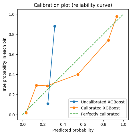
## Plot the calibration curves
plt.figure(figsize=(5, 5))
plt.plot(
   prob_pred_uncalibrated,
   prob_true_uncalibrated,
   marker="o",
   label="Uncalibrated XGBoost",
)
plt.plot(
   prob_pred_calibrated,
   prob_true_calibrated,
   marker="o",
   label="Calibrated XGBoost",
)
plt.plot(
   [0, 1],
   [0, 1],
   linestyle="--",
   label="Perfectly calibrated",
)
plt.xlabel("Predicted probability")
plt.ylabel("True probability in each bin")
plt.title("Calibration plot (reliability curve)")
plt.legend()
plt.show()

F1 Beta Threshold Tuning

In binary classification, selecting an optimal classification threshold is crucial for achieving the best balance between precision and recall. The default threshold of 0.5 may not always yield optimal performance, especially when dealing with imbalanced datasets. F1 Beta threshold tuning helps adjust this threshold to maximize the F-beta score, which balances precision and recall according to the importance assigned to each through the beta parameter.

Note

To better understand the impact of threshold tuning on model results, see the Threshold Tuning Considerations section.

Understanding F1 Beta Score

The F-beta score is a generalization of the F1-score that allows you to weigh recall more heavily than precision (or vice versa) based on the beta parameter:

F1-Score (beta = 1): Equal importance to precision and recall.
F-beta > 1: More emphasis on recall. Useful when false negatives are more critical (e.g., disease detection).
F-beta < 1: More emphasis on precision. Suitable when false positives are costlier (e.g., spam detection).

Example usage: default (beta = 1)

Setting up the Model object ready for tuning.

from xgboost import XGBClassifier

xgb_name = "xgb"
xgb = XGBClassifier(
   objective="binary:logistic"
   random_state=222,
)

tuned_parameters_xgb = {
   f"{xgb_name}__max_depth": [3, 10, 20, 200, 500],
   f"{xgb_name}__learning_rate": [1e-4],
   f"{xgb_name}__n_estimators": [1000],
   f"{xgb_name}__early_stopping_rounds": [100],
   f"{xgb_name}__verbose": [0],
   f"{xgb_name}__eval_metric": ["logloss"],
}

xgb_model = Model(
   name=f"Threshold Example Model",
   estimator_name=xgb_name,
   calibrate=False,
   model_type="classification",
   estimator=xgb,
   kfold=False,
   stratify_y=True,
   stratify_cols=False,
   grid=tuned_parameters_xgb,
   randomized_grid=False,
   boost_early=False,
   scoring=["roc_auc"],
   random_state=222,
   n_jobs=2,
)

In the grid_search_param_tuning use the f1_beta_tune variable when using grid_search_param_tuning(). Set this to True to enable tuning.

xgb_model.grid_search_param_tuning(X, y, f1_beta_tune=True)

This will find the best hyperparameters and then find the best threshold for these balancing both precision and recall. The threshold is stored in the Model object. To access this:

xgb_model.threshold

This will give the best threshold found for each score specified in the Model object.

When using methods to return metrics or report metrics and an optimal threshold was used make sure to remember to specify this in them for example:

xgb_model.return_metrics(
   X_valid,
   y_valid,
   optimal_threshold=True,
   print_threshold=True,
   model_metrics=True,
)

Example usage: custom betas (higher recall)

If we want to have a higher recall score and care less about precision then we increase the beta value. This looks very similar to the previous example except that when we use f1_beta_tune, we also set a beta value like so:

xgb_model.grid_search_param_tuning(X, y, f1_beta_tune=True, betas=[2])

Setting the beta value to 2 will priortise increasing the recall over the precision.

Example usage: custom betas (higher precision)

If we want to have a higher precision score and care less about recall then we decrease the beta value. This looks very similar to the previous example except that we set the beta value to less than 1.

xgb_model.grid_search_param_tuning(X, y, f1_beta_tune=True, betas=[0.5])

Setting the beta value to 0.5 will priortise increasing the precision over the recall.

Optimizing Model Threshold for Precision/Recall Trade-off

This function helps fine-tune a saved model’s decision threshold to maximize precision or recall using a beta-weighted approach.

Note

See this section for a more detailed explanation with contextual examples.

threshold, beta = find_optimal_threshold_beta(
   y_valid,
   model.predict_proba(X_valid)[:, 1],
   target_metric="precision",
   target_score=0.5,
   beta_value_range=np.linspace(0.01, 4, 40),
)

Imbalanced Learning

In machine learning, imbalanced datasets are a frequent challenge, especially in real-world scenarios. These datasets have an unequal distribution of target classes, with one class (e.g., fraudulent transactions, rare diseases, or other low-frequency events) being underrepresented compared to the majority class. Models trained on imbalanced data often struggle to generalize, as they tend to favor the majority class, leading to poor performance on the minority class.

To mitigate these issues, it is crucial to:

Understand the nature of the imbalance in the dataset.
Apply appropriate resampling techniques (oversampling, undersampling, or hybrid methods).
Use metrics beyond accuracy, such as precision, recall, and F1-score, to evaluate model performance fairly.

Generating an imbalanced dataset

Demonstrated below are the steps to generate an imbalanced dataset using make_classification from the sklearn.datasets module. The following parameters are specified:

n_samples=1000: The dataset contains 1,000 samples.
n_features=20: Each sample has 20 features.
n_informative=2: Two features are informative for predicting the target.
n_redundant=2: Two features are linear combinations of the informative features.
weights=[0.9, 0.1]: The target class distribution is 90% for the majority class and 10% for the minority class, creating an imbalance.
flip_y=0: No label noise is added to the target variable.
random_state=42: Ensures reproducibility by using a fixed random seed.

import pandas as pd
import numpy as np
from sklearn.datasets import make_classification

X, y = make_classification(
   n_samples=1000,
   n_features=20,
   n_informative=2,
   n_redundant=2,
   n_clusters_per_class=1,
   weights=[0.9, 0.1],
   flip_y=0,
   random_state=42,
)

## Convert to a pandas DataFrame for better visualization
data = pd.DataFrame(X, columns=[f'feature_{i}' for i in range(1, 21)])
data['target'] = y

X = data[[col for col in data.columns if "target" not in col]]
y = pd.Series(data["target"])

Below, you will see that the dataset we have generated is severely imbalanced with 900 observations allocated to the majority class (0) and 100 observations to the minority class (1).

import matplotlib.pyplot as plt

## Create a bar plot
value_counts = pd.Series(y).value_counts()
ax = value_counts.plot(
   kind="bar",
   rot=0,
   width=0.9,
)

## Add labels inside the bars
for index, count in enumerate(value_counts):
   plt.text(
      index,
      count / 2,
      str(count),
      ha="center",
      va="center",
      color="yellow",
   )

## Customize labels and title
plt.xlabel("Class")
plt.ylabel("Count")
plt.title("Class Distribution")

plt.show() ## Show the plot

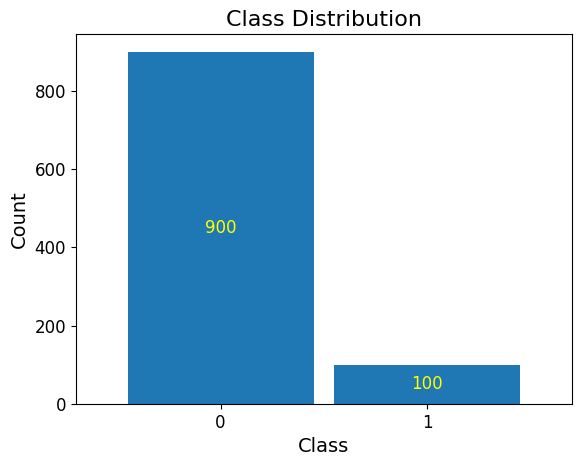
Define hyperparameters for XGBoost

Below, we will use an XGBoost classifier with the following hyperparameters:

from xgboost import XGBClassifier

xgb_name = "xgb"
xgb = XGBClassifier(
   random_state=222,
)
xgbearly = True

tuned_parameters_xgb = {
   f"{xgb_name}__max_depth": [3, 10, 20, 200, 500],
   f"{xgb_name}__learning_rate": [1e-4],
   f"{xgb_name}__n_estimators": [1000],
   f"{xgb_name}__early_stopping_rounds": [100],
   f"{xgb_name}__verbose": [0],
   f"{xgb_name}__eval_metric": ["logloss"],
}

xgb_definition = {
   "clc": xgb,
   "estimator_name": xgb_name,
   "tuned_parameters": tuned_parameters_xgb,
   "randomized_grid": False,
   "n_iter": 5,
   "early": xgbearly,
}

Define the model object

model_type = "xgb"
clc = xgb_definition["clc"]
estimator_name = xgb_definition["estimator_name"]

tuned_parameters = xgb_definition["tuned_parameters"]
n_iter = xgb_definition["n_iter"]
rand_grid = xgb_definition["randomized_grid"]
early_stop = xgb_definition["early"]
kfold = False
calibrate = True

Addressing Class Imbalance in Machine Learning

Class imbalance occurs when one class significantly outweighs another in the dataset, leading to biased models that perform well on the majority class but poorly on the minority class. Techniques like SMOTE and others aim to address this issue by improving the representation of the minority class, ensuring balanced learning and better generalization.

Techniques to Address Class Imbalance

Resampling Techniques

SMOTE (Synthetic Minority Oversampling Technique): SMOTE generates synthetic samples for the minority class by interpolating between existing minority class data points and their nearest neighbors. This helps create a more balanced class distribution without merely duplicating data, thus avoiding overfitting.
Oversampling: Randomly duplicates examples from the minority class to balance the dataset. While simple, it risks overfitting to the duplicated examples.
Undersampling: Reduces the majority class by randomly removing samples. While effective, it can lead to loss of important information.

Purpose of Using These Techniques

The goal of using these techniques is to improve model performance on imbalanced datasets, specifically by:

Ensuring the model captures meaningful patterns in the minority class.
Reducing bias toward the majority class, which often dominates predictions in imbalanced datasets.
Improving metrics like recall, F1-score, and AUC-ROC for the minority class, which are critical in applications like fraud detection, healthcare, and rare event prediction.

Note

While we provide comprehensive examples for SMOTE, ADASYN, and RandomUnderSampler in the accompanying notebook, this documentation section demonstrates the implementation of SMOTE. The other examples follow a similar workflow and can be executed by simply passing the respective imbalance_sampler input to ADASYN() or RandomUnderSampler(), as needed. For detailed examples of all methods, please refer to the linked notebook.

Synthetic Minority Oversampling Technique (SMOTE)

SMOTE (Synthetic Minority Oversampling Technique) is a method used to address class imbalance in datasets. It generates synthetic samples for the minority class by interpolating between existing minority samples and their nearest neighbors, effectively increasing the size of the minority class without duplicating data. This helps models better learn patterns from the minority class, improving classification performance on imbalanced datasets.

Step 1: Initalize and configure the model

Important

In the code block below, we initialize and configure the model by instantiating the Model class and assigning it to a variable named xgb_smote. Note that the imbalance_sampler=SMOTE(random_state=42) parameter is included to activate the imbalanced sampler. Setting a random state of 42 ensures reproducibility of results.

from model_tuner import Model
from imblearn.over_sampling import SMOTE

xgb_smote = Model(
   name=f"Make_Classification_{model_type}",
   estimator_name=estimator_name,
   calibrate=calibrate,
   model_type="classification",
   estimator=clc,
   kfold=kfold,
   stratify_y=True,
   stratify_cols=False,
   grid=tuned_parameters,
   randomized_grid=rand_grid,
   boost_early=early_stop,
   scoring=["roc_auc"],
   random_state=222,
   n_jobs=2,
   imbalance_sampler=SMOTE(random_state=42),
)

Step 2: Perform grid search parameter tuning and retrieve split data

xgb_smote.grid_search_param_tuning(X, y, f1_beta_tune=True)

## Get the training, validation, and test data
X_train, y_train = xgb_smote.get_train_data(X, y)
X_valid, y_valid = xgb_smote.get_valid_data(X, y)
X_test, y_test = xgb_smote.get_test_data(X, y)

Pipeline Steps:

┌─────────────────────┐
│ Step 1: resampler   │
│ SMOTE               │
└─────────────────────┘
         │
         ▼
┌─────────────────────┐
│ Step 2: xgb         │
│ XGBClassifier       │
└─────────────────────┘

Distribution of y values after resampling: target
0         540
1         540
Name: count, dtype: int64

100%|██████████| 5/5 [00:16<00:00,  3.25s/it]
Fitting model with best params and tuning for best threshold ...
100%|██████████| 2/2 [00:00<00:00,  4.17it/s]Best score/param set found on validation set:
{'params': {'xgb__early_stopping_rounds': 100,
            'xgb__eval_metric': 'logloss',
            'xgb__learning_rate': 0.0001,
            'xgb__max_depth': 3,
            'xgb__n_estimators': 999},
'score': 0.9969444444444445}
Best roc_auc: 0.997

SMOTE: Distribution of y values after resampling

Notice that the target has been redistributed after SMOTE to 540 observations for the minority class and 540 observations for the majority class.

Step 3: Fit the model

xgb_smote.fit(
   X_train,
   y_train,
   validation_data=[X_valid, y_valid],
)

Step 4: Return metrics (optional)

# ------------------------- VALID AND TEST METRICS -----------------------------

print("Validation Metrics")
xgb_smote.return_metrics(
   X_valid,
   y_valid,
   optimal_threshold=True,
   print_threshold=True,
   model_metrics=True,
)
print()

print("Test Metrics")
xgb_smote.return_metrics(
   X_test,
   y_test,
   optimal_threshold=True,
   print_threshold=True,
   model_metrics=True,
)

print()

Validation Metrics
Confusion matrix on set provided:
--------------------------------------------------------------------------------
         Predicted:
            Pos   Neg
--------------------------------------------------------------------------------
Actual: Pos  20 (tp)    0 (fn)
        Neg   1 (fp)  179 (tn)
--------------------------------------------------------------------------------
********************************************************************************
Report Model Metrics: xgb

            Metric     Value
0      Precision/PPV  0.952381
1  Average Precision  0.947751
2        Sensitivity  1.000000
3        Specificity  0.994444
4            AUC ROC  0.996944
5        Brier Score  0.208997
********************************************************************************
--------------------------------------------------------------------------------

              precision    recall  f1-score   support

           0       1.00      0.99      1.00       180
           1       0.95      1.00      0.98        20

    accuracy                           0.99       200
   macro avg       0.98      1.00      0.99       200
weighted avg       1.00      0.99      1.00       200

--------------------------------------------------------------------------------
Optimal threshold used: 0.52

Test Metrics
Confusion matrix on set provided:
--------------------------------------------------------------------------------
         Predicted:
            Pos   Neg
--------------------------------------------------------------------------------
Actual: Pos  18 (tp)    2 (fn)
        Neg   3 (fp)  177 (tn)
--------------------------------------------------------------------------------
********************************************************************************
Report Model Metrics: xgb

            Metric     Value
0      Precision/PPV  0.857143
1  Average Precision  0.897215
2        Sensitivity  0.900000
3        Specificity  0.983333
4            AUC ROC  0.966944
5        Brier Score  0.209358
********************************************************************************
--------------------------------------------------------------------------------

              precision    recall  f1-score   support

           0       0.99      0.98      0.99       180
           1       0.86      0.90      0.88        20

    accuracy                           0.97       200
   macro avg       0.92      0.94      0.93       200
weighted avg       0.98      0.97      0.98       200

--------------------------------------------------------------------------------
Optimal threshold used: 0.52

Recursive Feature Elimination (RFE)

Now that we’ve trained the models, we can also refine them by identifying which features contribute most to their performance. One effective method for this is Recursive Feature Elimination (RFE). This technique allows us to systematically remove the least important features, retraining the model at each step to evaluate how performance is affected. By focusing only on the most impactful variables, RFE helps streamline the dataset, reduce noise, and improve both the accuracy and interpretability of the final model.

It works by recursively training a model, ranking the importance of features based on the model’s outputas (such as coefficients in linear models or importance scores in tree-based models), and then removing the least important features one by one. This process continues until a specified number of features remains or the desired performance criteria are met.

The primary advantage of RFE is its ability to streamline datasets, improving model performance and interpretability by focusing on features that contribute the most to the predictive power. However, it can be computationally expensive since it involves repeated model training, and its effectiveness depends on the underlying model’s ability to evaluate feature importance. RFE is commonly used with cross-validation to ensure that the selected features generalize well across datasets, making it a robust choice for model optimization and dimensionality reduction.

As an illustrative example, we will retrain the above model using RFE.

from sklearn.feature_selection import RFE
from sklearn.linear_model import ElasticNet

We will begin by appending the feature selection technique to our tuned parameters dictionary.

xgb_definition["tuned_parameters"][f"feature_selection_rfe__n_features_to_select"] = [
   None,
   5,
   10,
]

Elastic Net for feature selection with RFE

Note

You may wish to explore this section for the rationale in applying this technique.

We will use elastic net because it strikes a balance between two widely used regularization techniques: Lasso (\(L1\)) and Ridge (\(L2\)). Elastic net is particularly effective in scenarios where we expect the dataset to have a mix of strongly and weakly correlated features. Lasso alone tends to select only one feature from a group of highly correlated ones, ignoring the others, while Ridge includes all features but may not perform well when some are entirely irrelevant. Elastic net addresses this limitation by combining both penalties, allowing it to handle multicollinearity more effectively while still performing feature selection.

Additionally, elastic net provides flexibility by controlling the ratio between \(L1\) and \(L2\) penalties, enabling fine-tuning to suit the specific needs of our dataset. This makes it a robust choice for datasets with many features, some of which may be irrelevant or redundant, as it can reduce overfitting while retaining a manageable subset of predictors.

rfe_estimator = ElasticNet(alpha=10.0, l1_ratio=0.9)

rfe = RFE(rfe_estimator)

from model_tuner import Model

model_xgb = Model(
   name=f"AIDS_Clinical_{model_type}",
   estimator_name=estimator_name,
   calibrate=calibrate,
   estimator=clc,
   model_type="classification",
   kfold=kfold,
   pipeline_steps=[
      ("rfe", rfe),
   ],
   stratify_y=True,
   stratify_cols=False,
   grid=tuned_parameters,
   randomized_grid=rand_grid,
   feature_selection=True,
   boost_early=early_stop,
   scoring=["roc_auc"],
   random_state=222,
   n_jobs=2,
)

model_xgb.grid_search_param_tuning(X, y, f1_beta_tune=True)

X_train, y_train = model_xgb.get_train_data(X, y)
X_valid, y_valid = model_xgb.get_valid_data(X, y)
X_test, y_test = model_xgb.get_test_data(X, y)

model_xgb.fit(
   X_train,
   y_train,
   validation_data=[X_valid, y_valid],
)


# ------------------------- VALID AND TEST METRICS -----------------------------

print("Validation Metrics")
model_xgb.return_metrics(
   X_valid,
   y_valid,
   optimal_threshold=True,
   print_threshold=True,
   model_metrics=True,
)
print()

print("Test Metrics")
model_xgb.return_metrics(
   X_test,
   y_test,
   optimal_threshold=True,
   print_threshold=True,
   model_metrics=True,
)

print()

Pipeline Steps:

┌─────────────────────────────────┐
│ Step 1: feature_selection_rfe   │
│ RFE                             │
└─────────────────────────────────┘
               │
               ▼
┌─────────────────────────────────┐
│ Step 2: xgb                     │
│ XGBClassifier                   │
└─────────────────────────────────┘

100%|██████████| 15/15 [00:40<00:00,  2.70s/it]
Fitting model with best params and tuning for best threshold ...
100%|██████████| 2/2 [00:00<00:00,  3.53it/s]
Best score/param set found on validation set:
{'params': {'feature_selection_rfe__n_features_to_select': 10,
            'xgb__early_stopping_rounds': 100,
            'xgb__eval_metric': 'logloss',
            'xgb__learning_rate': 0.0001,
            'xgb__max_depth': 10,
            'xgb__n_estimators': 999},
'score': 0.9324994064577399}
Best roc_auc: 0.932

Validation Metrics
Confusion matrix on set provided:
--------------------------------------------------------------------------------
         Predicted:
            Pos   Neg
--------------------------------------------------------------------------------
Actual: Pos  94 (tp)   10 (fn)
        Neg  70 (fp)  254 (tn)
--------------------------------------------------------------------------------
********************************************************************************
Report Model Metrics: xgb

            Metric     Value
0      Precision/PPV  0.573171
1  Average Precision  0.824825
2        Sensitivity  0.903846
3        Specificity  0.783951
4            AUC ROC  0.932499
5        Brier Score  0.165950
********************************************************************************
--------------------------------------------------------------------------------

              precision    recall  f1-score   support

           0       0.96      0.78      0.86       324
           1       0.57      0.90      0.70       104

    accuracy                           0.81       428
   macro avg       0.77      0.84      0.78       428
weighted avg       0.87      0.81      0.82       428

--------------------------------------------------------------------------------

Feature names selected:
['time', 'preanti', 'str2', 'strat', 'symptom', 'treat', 'offtrt', 'cd40', 'cd420', 'cd80']

Optimal threshold used: 0.25

Test Metrics
Confusion matrix on set provided:
--------------------------------------------------------------------------------
         Predicted:
            Pos   Neg
--------------------------------------------------------------------------------
Actual: Pos  93 (tp)   11 (fn)
        Neg  71 (fp)  253 (tn)
--------------------------------------------------------------------------------
********************************************************************************
Report Model Metrics: xgb

            Metric     Value
0      Precision/PPV  0.567073
1  Average Precision  0.817957
2        Sensitivity  0.894231
3        Specificity  0.780864
4            AUC ROC  0.930051
5        Brier Score  0.165771
********************************************************************************
--------------------------------------------------------------------------------

              precision    recall  f1-score   support

           0       0.96      0.78      0.86       324
           1       0.57      0.89      0.69       104

    accuracy                           0.81       428
   macro avg       0.76      0.84      0.78       428
weighted avg       0.86      0.81      0.82       428

--------------------------------------------------------------------------------

Feature names selected:
['time', 'preanti', 'str2', 'strat', 'symptom', 'treat', 'offtrt', 'cd40', 'cd420', 'cd80']

Optimal threshold used: 0.25

Important

Passing feature_selection=True in conjunction with accounting for rfe for the pipeline_steps inside the Model` class above is necessary to print the output of the feature names selected, thus yielding:

Feature names selected:
['time', 'preanti', 'str2', 'strat', 'symptom', 'treat', 'offtrt', 'cd40', 'cd420', 'cd80']

SHAP (SHapley Additive exPlanations)

This example demonstrates how to compute and visualize SHAP (SHapley Additive exPlanations) values for a machine learning model with a pipeline that includes feature selection. SHAP values provide insights into how individual features contribute to the predictions of a model.

Steps

The dataset is transformed through the model’s feature selection pipeline to ensure only the selected features are used for SHAP analysis.
The final model (e.g., XGBoost classifier) is retrieved from the custom Model object. This is required because SHAP operates on the underlying model, not the pipeline.
SHAP’s TreeExplainer is used to explain the predictions of the XGBoost classifier.
SHAP values are calculated for the transformed dataset to quantify the contribution of each feature to the predictions.
A summary plot is generated to visualize the impact of each feature across all data points.

Step 1: Transform the test data using the feature selection pipeline

## The pipeline applies preprocessing (e.g., imputation, scaling) and feature
## selection (RFE) to X_test
X_test_transformed = model_xgb.get_feature_selection_pipeline().transform(X_test)

Step 2: Retrieve the trained XGBoost classifier from the pipeline

## The last estimator in the pipeline is the XGBoost model
xgb_classifier = model_xgb.estimator[-1]

Step 3: Extract feature names from the training data, and initialize the SHAP explainer for the XGBoost classifier

## Import SHAP for model explainability
import shap

## Feature names are required for interpretability in SHAP plots
## If feature selection, Column Transformer or One Hot Encoders were used
feature_names = model.get_feature_names()

## Initialize the SHAP explainer with the model
explainer = shap.TreeExplainer(xgb_classifier)

Step 4: Compute SHAP values for the transformed test dataset and generate a summary plot of SHAP values

## Compute SHAP values for the transformed dataset
shap_values = explainer.shap_values(X_test_transformed)

Step 5: Generate a summary plot of SHAP values

## Plot SHAP values
## Summary plot of SHAP values for all features across all data points
shap.summary_plot(shap_values, X_test_transformed, feature_names=feature_names)

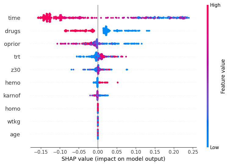
Feature Importance and Impact

This SHAP summary plot provides a detailed visualization of how each feature contributes to the model’s predictions, offering insight into feature importance and their directional effects. The X-axis represents SHAP values, which quantify the magnitude and direction of a feature’s influence. Positive SHAP values indicate that the feature increases the predicted output, while negative values suggest a decrease. Along the Y-axis, features are ranked by their overall importance, with the most influential features, such as time, positioned at the top.

Each point on the plot corresponds to an individual observation, where the color gradient reflects the feature value. Blue points represent lower feature values, while pink points indicate higher values, allowing us to observe how varying feature values affect the prediction. For example, the time feature shows a wide range of SHAP values, with higher values (pink) strongly increasing the prediction and lower values (blue) reducing it, demonstrating its critical role in driving the model’s output.

In contrast, features like hemo and age exhibit SHAP values closer to zero, signifying a lower overall impact on predictions. Features such as homo, karnof, and trt show more variability in their influence, indicating that their effect is context-dependent and can significantly shift predictions in certain cases. This plot provides a holistic view of feature behavior, enabling a deeper understanding of the model’s decision-making process.

Multi-Class Classification

Multi-class classification involves training a model to predict one of three or more distinct classes for each instance in a dataset. Unlike binary classification, where the model predicts between two classes (e.g., positive/negative), multi-class classification applies to problems where multiple outcomes exist, such as predicting the species of flowers in the Iris dataset.

This section demonstrates how to perform multi-class classification using the model_tuner library, with XGBoostClassifier as the base estimator and the Iris dataset as the example.

Iris Dataset with XGBoost

The Iris dataset is a benchmark dataset commonly used for multi-class classification. It contains 150 samples from three species of Iris flowers (Setosa, Versicolour, and Virginica), with four features: sepal length, sepal width, petal length, and petal width.

Step 1: Import Necessary Libraries

import pandas as pd
import numpy as np

from model_tuner.model_tuner_utils import Model, report_model_metrics
from sklearn.impute import SimpleImputer
from xgboost import XGBClassifier
from sklearn.pipeline import Pipeline
from sklearn.preprocessing import StandardScaler
from sklearn.compose import ColumnTransformer

from sklearn.datasets import load_iris

Step 2: Load the dataset. Define X, y

data = load_iris()
X = data.data
y = data.target


X = pd.DataFrame(X)
y = pd.DataFrame(y)

Step 3: Define the preprocessing steps

Preprocessing is a crucial step in machine learning workflows to ensure the input data is properly formatted and cleaned for the model. In this case, we define a preprocessing pipeline to handle scaling and missing values in numerical features. This ensures that the data is standardized and ready for training without introducing bias from inconsistent feature ranges or missing values.

The preprocessing pipeline consists of the following components:

Numerical Transformer: A pipeline that applies:
- StandardScaler for standardizing numerical features.
- SimpleImputer for imputing missing values with the mean strategy.
Column Transformer: Applies the numerical transformer to all columns and passes any remaining features through without transformation.

scalercols = X.columns

numerical_transformer = Pipeline(
    steps=[
        ("scaler", StandardScaler()),
        ("imputer", SimpleImputer(strategy="mean")),
    ]
)

# Create the ColumnTransformer with passthrough
preprocessor = ColumnTransformer(
    transformers=[
        ("num", numerical_transformer, scalercols),
    ],
    remainder="passthrough",
)

Step 4: Define the estimator and hyperparameters

In this step, we configure the XGBoostClassifier as the model estimator and define its hyperparameters for multi-class classification.

We use XGBClassifier with the objective="multi:softprob" parameter, which specifies multi-class classification using the softmax probability output.
Assign a name to the estimator for identification in the pipeline (e.g., xgb_mc for “XGBoost Multi-Class”).
Enable early stopping (early_stopping_rounds=20) to prevent overfitting by halting training if validation performance does not improve after 20 rounds.
Define a hyperparameter grid for tuning:
- max_depth: The maximum depth of a tree (e.g., 3, 10, 15).
- n_estimators: The number of boosting rounds (e.g., 5, 10, 15, 20).
- eval_metric: Evaluation metric (mlogloss for multi-class log-loss).
- verbose: Controls verbosity of output during training (1 = show progress).
- early_stopping_rounds: Number of rounds for early stopping.
Additional Configuration:
- Disable cross-validation (kfold=False) and calibration (calibrate=False).

estimator = XGBClassifier(objective="multi:softprob")

estimator_name = "xgb_mc"
xgbearly = True

tuned_parameters = {
    f"{estimator_name}__max_depth": [3, 10, 15],
    f"{estimator_name}__n_estimators": [5, 10, 15, 20],
    f"{estimator_name}__eval_metric": ["mlogloss"],
    f"{estimator_name}__verbose": [0],
    f"{estimator_name}__early_stopping_rounds": [20],
}

kfold = False
calibrate = False

Step 5: Initialize and configure the model

After defining the preprocessing steps and estimator, the next step is to initialize the Model class from the model_tuner library. This class brings together all essential components, including the preprocessing pipeline, estimator, hyperparameters, and scoring metrics, to streamline the model training and evaluation process.

The updated configuration includes:

Name and Type:
- Specify a descriptive name for the model (e.g., “XGB Multi Class”).
- Set the model_type to "classification" for multi-class classification.
Incorporate the preprocessor defined earlier using the ColumnTransformer, which handles scaling and imputation for numerical features.
Estimator and Hyperparameters:
- Link the estimator_name to the hyperparameter grid defined earlier (tuned_parameters).
- Pass the XGBClassifier as the estimator.
Early Stopping and Cross-Validation:
- Enable early stopping with boost_early=True.
- Disable cross-validation with kfold=False.
Additional Configurations:
- Use stratify_y=True for stratified splits.
- Set multi_label=True to enable multi-class classification.
- Use roc_auc_ovr (One-vs-Rest ROC AUC) as the scoring metric.
- Specify the class labels for the Iris dataset (["1", "2", "3"]).

model_xgb = Model(
    name="XGB Multi Class",
    model_type="classification",
    estimator_name=estimator_name,
    pipeline_steps=[("ColumnTransformer", preprocessor)],
    calibrate=calibrate,
    estimator=estimator,
    kfold=kfold,
    stratify_y=True,
    boost_early=xgbearly,
    grid=tuned_parameters,
    multi_label=True,
    randomized_grid=False,
    n_iter=4,
    scoring=["roc_auc_ovr"],
    n_jobs=-2,
    random_state=42,
    class_labels=["1", "2", "3"],
)

Step 6: Perform grid search parameter tuning

With the model configured, the next step is to perform grid search parameter tuning to find the optimal hyperparameters for the XGBClassifier. The grid_search_param_tuning method will iterate over all combinations of hyperparameters specified in tuned_parameters, evaluate each one using the specified scoring metric, and select the best performing set.

This method will:

Split the Data: The data will be split into training and validation sets. Since stratify_y=True, the class distribution will be maintained across splits.
Iterate Over Hyperparameters: All combinations of hyperparameters defined in tuned_parameters will be tried since randomized_grid=False.
Early Stopping: With boost_early=True and early_stopping_rounds set in the hyperparameters, the model will stop training early if the validation score does not improve.
Scoring: The model uses roc_auc_ovr (One-vs-Rest ROC AUC) as the scoring metric suitable for multi-class classification.
Select Best Model: The hyperparameter set that yields the best validation score will be selected.

To execute the grid search, simply call:

model.grid_search_param_tuning(X, y)

Pipeline Steps:

┌───────────────────────────────────────────────────────────┐
│ Step 1: preprocess_column_transformer_ColumnTransformer   │
│ ColumnTransformer                                         │
└───────────────────────────────────────────────────────────┘
                           │
                           ▼
┌───────────────────────────────────────────────────────────┐
│ Step 2: xgb_mc                                            │
│ XGBClassifier                                             │
└───────────────────────────────────────────────────────────┘

100%|██████████| 12/12 [00:00<00:00, 22.10it/s]Best score/param set found on validation set:
{'params': {'xgb_mc__early_stopping_rounds': 20,
            'xgb_mc__eval_metric': 'mlogloss',
            'xgb_mc__max_depth': 10,
            'xgb_mc__n_estimators': 10},
'score': 0.9666666666666668}
Best roc_auc_ovr: 0.967

Step 7: Generate data splits

Once the best hyperparameters are identified through grid search, the next step is to generate the training, validation, and test splits. The Model class provides built-in methods for creating these splits while maintaining the class distribution (as specified by stratify_y=True).

Use the following code to generate the splits:

## Get the training, validation, and test data
X_train, y_train = model_xgb.get_train_data(X, y)
X_valid, y_valid = model_xgb.get_valid_data(X, y)
X_test, y_test = model_xgb.get_test_data(X, y)

Description of Splits:

Training Data (X_train, y_train): Used to train the model.
Validation Data (X_valid, y_valid): Used during training for monitoring and fine-tuning, including techniques like early stopping.
Test Data (X_test, y_test): Reserved for evaluating the final performance of the trained model.

These splits ensure that each phase of model development (training, validation, and testing) is performed on separate portions of the dataset, providing a robust evaluation pipeline.

Step 8: Fit the model

After generating the data splits, the next step is to train the model using the training data and validate its performance on the validation data during training. The fit method in the Model class handles this process seamlessly, leveraging the best hyperparameters found during grid search.

Use the following code to fit the model:

model_xgb.fit(
    X_train,
    y_train,
    validation_data=[X_valid, y_valid],
)

Note

Training Data (X_train, y_train): The model is trained on this data to learn patterns.
Validation Data (X_valid, y_valid): During training, the model monitors its performance on this data to avoid overfitting and apply techniques like early stopping.
Early Stopping: If boost_early=True and early_stopping_rounds is defined, training will halt early when validation performance stops improving.

This step ensures that the model is fitted using the best configuration from the grid search and optimized for generalization. With the model trained, proceed to Step 9 to evaluate its performance on validation and test datasets.

Step 9: Return metrics (optional)

Once the model is trained, you can evaluate its performance on the validation and test datasets by returning key metrics. The return_metrics method from the Model class calculates and displays metrics like ROC AUC, precision, recall, and F1-score.

Use the following code to return metrics:

# Evaluate on validation data
print("Validation Metrics")
model_xgb.return_metrics(
   X_valid,
   y_valid,
   optimal_threshold=True,
)

# Predict probabilities for the test data
y_prob = model.predict_proba(X_test)

# Evaluate on test data
print("Test Metrics")
model_xgb.return_metrics(
   X_test,
   y_test,
   optimal_threshold=True,
)

Validation Metrics
--------------------------------------------------------------------------------
1
         Predicted:
            Pos  Neg
--------------------------------------------------------------------------------
Actual: Pos 19 (tn)   1 (fp)
        Neg  0 (fn)  10 (tp)
--------------------------------------------------------------------------------
2
         Predicted:
            Pos  Neg
--------------------------------------------------------------------------------
Actual: Pos 19 (tn)   1 (fp)
        Neg  2 (fn)   8 (tp)
--------------------------------------------------------------------------------
3
         Predicted:
            Pos  Neg
--------------------------------------------------------------------------------
Actual: Pos 19 (tn)   1 (fp)
        Neg  1 (fn)   9 (tp)
--------------------------------------------------------------------------------

              precision    recall  f1-score   support

           0       0.91      1.00      0.95        10
           1       0.89      0.80      0.84        10
           2       0.90      0.90      0.90        10

    accuracy                           0.90        30
   macro avg       0.90      0.90      0.90        30
weighted avg       0.90      0.90      0.90        30

--------------------------------------------------------------------------------
Test Metrics
--------------------------------------------------------------------------------
1
         Predicted:
            Pos  Neg
--------------------------------------------------------------------------------
Actual: Pos 18 (tn)   2 (fp)
        Neg  0 (fn)  10 (tp)
--------------------------------------------------------------------------------
2
         Predicted:
            Pos  Neg
--------------------------------------------------------------------------------
Actual: Pos 19 (tn)   1 (fp)
        Neg  2 (fn)   8 (tp)
--------------------------------------------------------------------------------
3
         Predicted:
            Pos  Neg
--------------------------------------------------------------------------------
Actual: Pos 20 (tn)   0 (fp)
        Neg  1 (fn)   9 (tp)
--------------------------------------------------------------------------------

              precision    recall  f1-score   support

           0       0.83      1.00      0.91        10
           1       0.89      0.80      0.84        10
           2       1.00      0.90      0.95        10

    accuracy                           0.90        30
   macro avg       0.91      0.90      0.90        30
weighted avg       0.91      0.90      0.90        30

--------------------------------------------------------------------------------
{'Classification Report': {'0': {'precision': 0.8333333333333334,
   'recall': 1.0,
   'f1-score': 0.9090909090909091,
   'support': 10.0},
'1': {'precision': 0.8888888888888888,
   'recall': 0.8,
   'f1-score': 0.8421052631578948,
   'support': 10.0},
'2': {'precision': 1.0,
   'recall': 0.9,
   'f1-score': 0.9473684210526316,
   'support': 10.0},
'accuracy': 0.9,
'macro avg': {'precision': 0.9074074074074074,
   'recall': 0.9,
   'f1-score': 0.8995215311004786,
   'support': 30.0},
'weighted avg': {'precision': 0.9074074074074073,
   'recall': 0.9,
   'f1-score': 0.8995215311004785,
   'support': 30.0}},
'Confusion Matrix': array([[[18,  2],
        [ 0, 10]],

       [[19,  1],
        [ 2,  8]],

       [[20,  0],
        [ 1,  9]]])}

Report Model Metrics

You can summarize and display the model’s performance metrics using the report_model_metrics function. This function computes key metrics like precision, recall, F1-score, and ROC AUC for each class, as well as macro and weighted averages.

Use the following code:

metrics_df = report_model_metrics(
   model=model_xgb,
   X_valid=X_test,
   y_valid=y_test,
   threshold=next(iter(model_xgb.threshold.values())),
)
print(metrics_df)

0 Precision/PPV                  0.833333
0 Sensitivity/Recall             1.000000
0 F1-Score                       0.909091
1 Precision/PPV                  0.888889
1 Sensitivity/Recall             0.800000
1 F1-Score                       0.842105
2 Precision/PPV                  1.000000
2 Sensitivity/Recall             0.900000
2 F1-Score                       0.947368
macro avg Precision/PPV          0.907407
macro avg Sensitivity/Recall     0.900000
macro avg F1-Score               0.899522
weighted avg Precision/PPV       0.907407
weighted avg Sensitivity/Recall  0.900000
weighted avg F1-Score            0.899522
Weighted Average Precision       0.907407
Weighted Average Recall          0.900000
Multiclass AUC ROC               0.933333

Note

Validation Metrics: Provide insights into how well the model performed during training and tuning on unseen validation data.
Test Metrics: Assess the final model’s generalization performance on completely unseen test data.
predict_proba: Outputs the predicted probabilities for each class, useful for calculating metrics like ROC AUC or understanding the model’s confidence in its predictions.

By examining these metrics, you can evaluate the model’s strengths and weaknesses and determine if further fine-tuning or adjustments are necessary.

Step 10: Predict probabilities and generate predictions

As an additional step, you can use the trained model to predict probabilities and generate predictions for the test data. This is particularly useful for analyzing model outputs or evaluating predictions with custom thresholds.

Use the following code:

## Predict probabilities for the test data
y_prob = model.predict_proba(X_test)[:, 1]

## Predict class labels using the optimal threshold
y_pred = model.predict(X_test, optimal_threshold=True)

# Print results
print(f"Predicted Probabilities: \n {y_prob}")
print()
print(f"Predictions: \n {y_pred}")

Predicted Probabilities:
[0.961671   0.02298635 0.749543   0.02298635 0.0244073  0.02298635
0.94500786 0.02298635 0.0227305  0.02298635 0.14078036 0.32687086
0.94500786 0.961671   0.95576227 0.02298635 0.02298635 0.02298635
0.961671   0.0244073  0.0227305  0.02298635 0.02298635 0.38560066
0.02298635 0.02298635 0.961671   0.0227305  0.0227305  0.4547262 ]

Predictions:
[1 0 1 0 0 0 1 0 0 0 0 0 1 1 1 0 0 0 1 0 0 0 0 0 0 0 1 0 0 0]

Note

Predicted Probabilities (predict_proba): Returns the probabilities for each class. The [:, 1] selects the probabilities for the second class (or one of interest).
Predicted Labels (predict): Generates class predictions using the optimal threshold, which is tuned during grid search or based on the scoring metric.
Optimal Threshold: When optimal_threshold=True, the model uses the threshold that maximizes a selected performance metric (e.g., F1-score or ROC AUC) instead of the default threshold of 0.5.
Analysis: Inspecting probabilities and predictions helps to interpret the model’s confidence and accuracy in making decisions.

This step allows for a deeper understanding of the model’s predictions and can be used to fine-tune decision thresholds or evaluate specific cases.

Regression

Here is an example of using the Model class for a regression task with XGBoost on the California Housing dataset.

The California Housing dataset, available in the sklearn library, is a commonly used benchmark dataset for regression problems. It contains features such as median income, housing age, and population, which are used to predict the median house value for California districts.

In this example, we leverage the Model class to:

Set up an XGBoost regressor as the estimator.
Define a hyperparameter grid for tuning the model.
Preprocess the dataset, train the model, and evaluate its performance using the \(R^2\) metric.

The workflow highlights how the Model class simplifies regression tasks, including hyperparameter tuning, and performance evaluation.

California Housing with XGBoost

Step 1: Import necessary libraries

import pandas as pd
import numpy as np
from xgboost import XGBRegressor
from sklearn.impute import SimpleImputer
from sklearn.datasets import fetch_california_housing
from model_tuner import Model

Step 2: Load the dataset

## Load the California Housing dataset
data = fetch_california_housing()
X = pd.DataFrame(data.data, columns=data.feature_names)
y = pd.Series(data.target, name="target")

Step 3: Create an instance of the XGBRegressor

xgb_name = "xgb"
xgb = XGBRegressor(random_state=222)

Step 4: Define Hyperparameters for XGBRegressor

In this step, we configure the XGBRegressor for a regression task. The hyperparameter grid includes key settings to control the learning process, tree construction, and generalization performance of the model.

The hyperparameter grid and model configuration are defined as follows:

tuned_parameters_xgb = [
    {
        f"{xgb_name}__learning_rate": [0.1, 0.01, 0.05],
        f"{xgb_name}__n_estimators": [100, 200, 300],
        f"{xgb_name}__max_depth": [3, 5, 7][:1],
        f"{xgb_name}__subsample": [0.8, 1.0][:1],
        f"{xgb_name}__colsample_bytree": [0.8, 1.0][:1],
        f"{xgb_name}__eval_metric": ["logloss"],
        f"{xgb_name}__early_stopping_rounds": [10],
        f"{xgb_name}__tree_method": ["hist"],
        f"{xgb_name}__verbose": [0],
    }
]
xgb_definition = {
    "clc": xgb,
    "estimator_name": xgb_name,
    "tuned_parameters": tuned_parameters_xgb,
    "randomized_grid": False,
    "early": True,
}

model_definition = {xgb_name: xgb_definition}

Key Configurations

learning_rate: Controls the contribution of each boosting round to the final prediction.
n_estimators: Specifies the total number of boosting rounds (trees).
max_depth: Limits the depth of each tree to prevent overfitting.
subsample: Fraction of training data used for fitting each tree, introducing randomness to improve generalization.
colsample_bytree: Fraction of features considered for each boosting round.
eval_metric: Specifies the evaluation metric to monitor during training (e.g., "logloss").
early_stopping_rounds: Stops training if validation performance does not improve for a set number of rounds.
tree_method: Chooses the algorithm used for tree construction ("hist" for histogram-based methods, optimized for speed).
verbose: Controls output display during training (set to 0 for silent mode).

Step 5: Initialize and configure the `Model`

XGBRegressor inherently handles missing values (NaN) without requiring explicit imputation strategies. During training, XGBoost treats missing values as a separate category and learns how to route them within its decision trees. Therefore, passing a SimpleImputer or using an imputation strategy is unnecessary when using XGBRegressor.

kfold = False
calibrate = False

## Define model object
model_type = "xgb"
clc = model_definition[model_type]["clc"]
estimator_name = model_definition[model_type]["estimator_name"]

## Set the parameters by cross-validation
tuned_parameters = model_definition[model_type]["tuned_parameters"]
rand_grid = model_definition[model_type]["randomized_grid"]
early_stop = model_definition[model_type]["early"]

model_xgb = Model(
   name=f"xgb_{model_type}",
   estimator_name=estimator_name,
   model_type="regression",
   calibrate=calibrate,
   estimator=clc,
   kfold=kfold,
   stratify_y=False,
   grid=tuned_parameters,
   randomized_grid=rand_grid,
   boost_early=early_stop,
   scoring=["r2"],
   random_state=222,
   n_jobs=2,
)

Step 6: Perform grid search parameter tuning and retrieve split data

To execute the grid search, simply call:

model_xgb.grid_search_param_tuning(X, y)

## Get the training, validation, and test data
X_train, y_train = model_xgb.get_train_data(X, y)
X_valid, y_valid = model_xgb.get_valid_data(X, y)
X_test, y_test = model_xgb.get_test_data(X, y)

With the model configured, the next step is to perform grid search parameter tuning to find the optimal hyperparameters for the XGBRegressor. The grid_search_param_tuning method will iterate over all combinations of hyperparameters specified in tuned_parameters_xgb, evaluate each one using the specified scoring metric, and select the best performing set.

This method will:

Split the Data: The data will be split into training and validation sets. Since stratify_y=False, the class distribution will not be maintained across splits.
Iterate Over Hyperparameters: All combinations of hyperparameters defined in tuned_parameters_xgb will be tried since randomized_grid=False.
Early Stopping: With boost_early=True and early_stopping_rounds set in the hyperparameters, the model will stop training early if the validation score does not improve.
Scoring: The model uses \(R^2\) as the scoring metric, which is suitable for evaluating regression models.
Select Best Model: The hyperparameter set that yields the best validation score based on the specified metric (\(R^2\)) will be selected.

Pipeline Steps:

┌────────────────┐
│ Step 1: xgb    │
│ XGBRegressor   │
└────────────────┘

100%|██████████| 9/9 [00:22<00:00,  2.45s/it]Best score/param set found on validation set:
{'params': {'xgb__colsample_bytree': 0.8,
            'xgb__early_stopping_rounds': 10,
            'xgb__eval_metric': 'logloss',
            'xgb__learning_rate': 0.1,
            'xgb__max_depth': 3,
            'xgb__n_estimators': 67,
            'xgb__subsample': 0.8,
            'xgb__tree_method': 'hist'},
'score': 0.7651490279157868}
Best r2: 0.765

Step 7: Fit the model

model_xgb.fit(
   X_train,
   y_train,
   validation_data=[X_valid, y_valid],
)

Step 8: Return metrics (optional)

Validation Metrics
********************************************************************************
{'Explained Variance': 0.7647451659057567,
'Mean Absolute Error': 0.3830825326824073,
'Mean Squared Error': 0.3066172248224347,
'Median Absolute Error': 0.2672762813568116,
'R2': 0.7647433075624044,
'RMSE': 0.5537302816556403}
********************************************************************************
Test Metrics
********************************************************************************
{'Explained Variance': 0.7888942913974833,
'Mean Absolute Error': 0.3743548199982513,
'Mean Squared Error': 0.28411432705731066,
'Median Absolute Error': 0.26315186452865597,
'R2': 0.7888925135381788,
'RMSE': 0.533023758436067}
********************************************************************************
{'Explained Variance': 0.7888942913974833,
'R2': 0.7888925135381788,
'Mean Absolute Error': 0.3743548199982513,
'Median Absolute Error': 0.26315186452865597,
'Mean Squared Error': 0.28411432705731066,
'RMSE': 0.533023758436067}

Performance Evaluation Metrics

Using `report_model_metrics()`

The report_model_metrics() method provides detailed insights into model performance, including metrics such as precision, recall, sensitivity, specificity, and AUC-ROC. For regression models, it includes key metrics such as Mean Absolute Error (MAE), Mean Squared Error (MSE), Root Mean Squared Error (RMSE), R² Score, and Explained Variance.

While this method is integrated into return_metrics(), it can also be invoked independently for custom evaluation workflows. For example, it can be used to focus on specific metrics or to analyze a subset of the data.

Using `return_metrics()`

A key feature of return_metrics() is its ability to retrieve and print the threshold value used to train the model. This threshold can be passed directly into report_model_metrics() for consistent evaluation.

Threshold Tuning

Model thresholding is a critical concept in classification tasks, allowing you to fine-tune the decision boundary for predicting positive or negative classes. Instead of relying on the default threshold of 0.5, which may not suit all datasets or evaluation metrics, thresholds can be adjusted to optimize metrics like precision, recall, or F1-score based on your specific objectives.

The model.threshold attribute provides a dictionary where each scoring metric is paired with its corresponding optimal threshold, enabling precise control over predictions. This is particularly useful in applications where the cost of false positives and false negatives differs significantly.

For example:

## Accessing the optimal thresholds for each scoring metric
print(model_xgb.threshold)

{'roc_auc': 0.25}

When to Use Custom Thresholds:

Imbalanced Datasets: Adjusting thresholds can help mitigate the effects of class imbalance by prioritizing recall or precision for the minority class.
Domain-Specific Goals: In medical diagnostics, for instance, you might prefer a lower threshold to maximize sensitivity (recall) and minimize false negatives.
Optimizing for Specific Metrics: If your primary evaluation metric is F-beta, tuning the threshold ensures better alignment with your goals.

How to Automatically Tune Thresholds

The optimal threshold can be automatically tuned by enabling F-beta optimization during parameter tuning. This can be done by setting f1_beta_tune=True in the grid_search_param_tuning() method:

# Automatically tune thresholds for F-beta optimization
model_xgb.grid_search_param_tuning(X, y, f1_beta_tune=True)

After tuning, the optimal thresholds will be stored in the model.threshold attribute for each scoring metric:

## Retrieve the optimal threshold for a specific metric
threshold = model_xgb.threshold['roc_auc']

Using threshold in `report_model_metrics()`

After calling return_metrics() with optimal_threshold=True, you can reuse the threshold in report_model_metrics() as shown below:

threshold = model_xgb.threshold['roc_auc']  # Retrieve the optimal threshold
model_xgb.report_model_metrics(X=X_valid, y=y_valid, threshold=threshold)

Reporting Threshold in `return_metrics`

The return_metrics method provides the flexibility to retrieve and print the threshold used during model evaluation, enabling seamless reuse in other methods or manual experimentation. When print_threshold=True is specified, the threshold will be included as part of the output, making it easy to reference and apply in subsequent analyses.

Example:

# Retrieve metrics and threshold using return_metrics
model_xgb.return_metrics(
    X=X_valid,
    y=y_valid,
    optimal_threshold=True,
    print_threshold=True,
    model_metrics=True
)

By including print_threshold=True, the optimal threshold used for predictions is displayed, ensuring transparency and providing a valuable reference for further evaluations or custom workflows.

Classification report (optional)

A call to print(model_xgb.classification_report) will output the classification report as follows:

print(model_xgb.classification_report)

              precision    recall  f1-score   support

           0       0.91      0.94      0.92       324
           1       0.79      0.71      0.75       104

    accuracy                           0.88       428
   macro avg       0.85      0.82      0.84       428
weighted avg       0.88      0.88      0.88       428

Bootstrap Metrics

The bootstrapper.py module provides utility functions for input type checking, data resampling, and evaluating bootstrap metrics.

check_input_type(x)

Validates and normalizes the input type for data processing. Converts NumPy arrays, Pandas Series, and DataFrames into a standard Pandas DataFrame with a reset index.

Parameters:: x (array-like) – Input data (NumPy array, Pandas Series, or DataFrame).
Returns:: Normalized input as a Pandas DataFrame.
Return type:: pandas.DataFrame
Raises:: ValueError – If the input type is not supported.

sampling_method(y, n_samples, stratify=False, balance=False, class_proportions=None)

Resamples a dataset based on specified options for balancing, stratification, or custom class proportions.

Parameters:

y (pandas.Series) – Target variable to resample.
n_samples (int) – Number of samples to draw.
stratify (bool, optional) – Whether to stratify based on the provided target variable.
balance (bool, optional) – Whether to balance class distributions equally.
class_proportions (dict, optional) – Custom proportions for each class. Must sum to 1.

Returns:

Resampled target variable.

Return type:

pandas.DataFrame

Raises:

ValueError – If class proportions do not sum to 1.

evaluate_bootstrap_metrics(model=None, X=None, y=None, y_pred_prob=None, n_samples=500, num_resamples=1000, metrics=['roc_auc', 'f1_weighted', 'average_precision'], random_state=42, threshold=0.5, model_type='classification', stratify=None, balance=False, class_proportions=None)

Evaluates classification or regression metrics on bootstrap samples using a pre-trained model or pre-computed predictions.

Parameters:

model (object, optional) – Pre-trained model with a predict_proba method. Required if y_pred_prob is not provided.
X (array-like, optional) – Input features. Not required if y_pred_prob is provided.
y (array-like) – Ground truth labels.
y_pred_prob (array-like, optional) – Pre-computed predicted probabilities.
n_samples (int, optional) – Number of samples per bootstrap iteration. Default is 500.
num_resamples (int, optional) – Number of bootstrap iterations. Default is 1000.
metrics (list of str) – List of metrics to calculate (e.g., "roc_auc", "f1_weighted").
random_state (int, optional) – Random seed for reproducibility. Default is 42.
threshold (float, optional) – Classification threshold for probability predictions. Default is 0.5.
model_type (str) – Specifies the task type, either "classification" or "regression".
stratify (pandas.Series, optional) – Variable for stratified sampling.
balance (bool, optional) – Whether to balance class distributions.
class_proportions (dict, optional) – Custom class proportions for sampling.

Returns:

DataFrame with mean and confidence intervals for each metric.

Return type:

pandas.DataFrame

Raises:

ValueError – If invalid parameters or metrics are provided.
RuntimeError – If sample size is insufficient for metric calculation.

Note

The model_tuner_utils.py module includes utility functions for evaluating bootstrap metrics in the context of model tuning.

return_bootstrap_metrics(X_test, y_test, metrics, threshold=0.5, num_resamples=500, n_samples=500, balance=False)

Evaluates bootstrap metrics for a trained model using the test dataset. This function supports both classification and regression tasks by leveraging evaluate_bootstrap_metrics to compute confidence intervals for the specified metrics.

Parameters:

X_test (pandas.DataFrame) – Test dataset features.
y_test (pandas.Series or pandas.DataFrame) – Test dataset labels.
metrics (list of str) – List of metric names to calculate (e.g., "roc_auc", "f1_weighted").
threshold (float, optional) – Threshold for converting predicted probabilities into class predictions. Default is 0.5.
num_resamples (int, optional) – Number of bootstrap iterations. Default is 500.
n_samples (int, optional) – Number of samples per bootstrap iteration. Default is 500.
balance (bool, optional) – Whether to balance the class distribution during resampling. Default is False.

Returns:

DataFrame containing mean and confidence intervals for the specified metrics.

Return type:

pandas.DataFrame

Raises:

ValueError – If X_test or y_test are not provided as Pandas DataFrames or if unsupported input types are specified.

Bootstrap metrics example

Continuing from the model output object (model_xgb) from the regression example above, we leverage the return_bootstrap_metrics method from model_tuner_utils.py to print bootstrap performance metrics (\(R^2\) and \(\text{explained variance}\)) at 95% confidence levels as shown below:

print("Bootstrap Metrics")

model_xgb.return_bootstrap_metrics(
   X_test=X_test,
   y_test=y_test,
   metrics=["r2", "explained_variance"],
   n_samples=30,
   num_resamples=300,
)

Bootstrap Metrics
100%|██████████| 300/300 [00:00<00:00, 358.05it/s]
Metric                     Mean  95% CI Lower  95% CI Upper
0                 r2   0.781523      0.770853      0.792193
1 explained_variance   0.788341      0.777898      0.798785

iPython Notebooks

Binary Classification Examples

Regression Example

Input Parameters

Key Methods and Functionalities

__init__(...)

reset_estimator()

process_imbalance_sampler()

calibrateModel()

Get train, val, test data

get_train_data()

get_valid_data()

get_test_data()

calibrate_report()

fit()

return_metrics()

predict()

grid_search_param_tuning()

print_selected_best_features()

tune_threshold_Fbeta()

train_val_test_split()

get_best_score_params()

conf_mat_class_kfold()

regression_report_kfold()

regression_report()

report_model_metrics()

find_optimal_threshold_beta()

Helper Functions

kfold_split()

get_cross_validate()

_confusion_matrix_print()

print_pipeline()

Pipeline Management

Specifying Pipeline Steps

Helper Methods for Pipeline Extraction

Extracting Feature names

Summary

Binary Classification

AIDS Clinical Trials Group Study

Step 1: Import Necessary libraries

Step 2: Load the dataset, define X, y

Step 3: Check for zero-variance columns and drop accordingly

Step 4: Create an instance of the XGBClassifier

Step 5: Define Hyperparameters for XGBoost

Step 6: Initialize and configure the Model

Step 7: Perform grid search parameter tuning and retrieve split data

Step 8: Fit the model

Step 9: Return metrics (optional)

Step 10: Calibrate the model (if needed)

F1 Beta Threshold Tuning

Understanding F1 Beta Score

Example usage: default (beta = 1)

Example usage: custom betas (higher recall)

Example usage: custom betas (higher precision)

Optimizing Model Threshold for Precision/Recall Trade-off

Imbalanced Learning

Generating an imbalanced dataset

Define hyperparameters for XGBoost

Define the model object

Addressing Class Imbalance in Machine Learning

Techniques to Address Class Imbalance

Purpose of Using These Techniques

Synthetic Minority Oversampling Technique (SMOTE)

Step 1: Initalize and configure the model

Step 2: Perform grid search parameter tuning and retrieve split data

SMOTE: Distribution of y values after resampling

Step 3: Fit the model

Step 4: Return metrics (optional)

Recursive Feature Elimination (RFE)

Elastic Net for feature selection with RFE

SHAP (SHapley Additive exPlanations)

Step 1: Transform the test data using the feature selection pipeline

Step 2: Retrieve the trained XGBoost classifier from the pipeline

Step 3: Extract feature names from the training data, and initialize the SHAP explainer for the XGBoost classifier

Step 4: Compute SHAP values for the transformed test dataset and generate a summary plot of SHAP values

Step 5: Generate a summary plot of SHAP values

Feature Importance and Impact

Multi-Class Classification

Iris Dataset with XGBoost

Step 1: Import Necessary Libraries

`init(...)`

`reset_estimator()`

`process_imbalance_sampler()`

`calibrateModel()`

`get_train_data()`

`get_valid_data()`

`get_test_data()`

`calibrate_report()`

`fit()`

`return_metrics()`

`predict()`

`grid_search_param_tuning()`

`print_selected_best_features()`

`tune_threshold_Fbeta()`

`train_val_test_split()`

`get_best_score_params()`

`conf_mat_class_kfold()`

`regression_report_kfold()`

`regression_report()`

`report_model_metrics()`

`find_optimal_threshold_beta()`

`kfold_split()`

`get_cross_validate()`

`_confusion_matrix_print()`

`print_pipeline()`

Step 6: Initialize and configure the `Model`

Step 5: Initialize and configure the `Model`

Using `report_model_metrics()`

Using `return_metrics()`

Using threshold in `report_model_metrics()`

Reporting Threshold in `return_metrics`